
|
|
|
|
|
This tutorial illustrates some techniques to navigate through challenges of bringing a theoretical quantum algorithm to the reality of NISQ devices. Quantum Chess serves as an example to demonstrate these ideas without some of the domain knowledge needed in other experiments.
This tutorial assumes basic knowledge of the following:
- Basic quantum computing principles, specifically, what unitary matrices are, and what an \(\text{iSWAP}\) (and \(\sqrt{\text{iSWAP} }\) gate is)
- The basic movement rules of Chess and the Algebraic notation method of naming chess squares and moves.
- The Cirq framework for constructing quantum circuits.
- While the tutorial will briefly cover the rules of quantum chess, those who are unfamiliar with this game may try it out or read the exact rules in the Quantum Chess paper. You can also find a sample implementation in this repository under
unitary.quantum_chess.
The goal of this tutorial is to illustrate some basic ideas of transforming a theoretical algorithm (such as Quantum Chess) into a real hardware algorithm, without getting lost in details of more complicated domain-specific problems.
The tutorial is split into several parts:
- Introduction to Quantum Chess: how quantum chess maps to qubits and quantum operations
- Quantum chess in Cirq: how to execute these operations using the cirq framework
- Handling partial measurement: how to handle moves that include measurement that partially collapses the board state
- Noise: how to deal with some simple noise models
- Decomposition: how to decompose gates
- Qubit Layout: how to run circuits when connectivity matters.
You will learn about the concepts of circuit construction, post-selection, gate decomposition, noise, optimizers, and qubit mappings.
First, let's get started by installing cirq on our colab runtime:
try:
    import unitary
except ImportError:
    !pip install --quiet git+https://github.com/quantumlib/unitary
import cirq
import cirq_google
from typing import Dict, Iterable, Optional, Set
Introduction to Quantum Chess
Quantum chess is analogous to the classical game of Chess. Special rules are added to the game in order to allow for superposition and entanglement of pieces. This tutorial will go over the basics of the rules in order to show how one might implement them in cirq and convert them to use a hardware device. The full rule set, including rules for more complicated situations (such as castling and en passant) can be found in the Quantum Chess paper. A demo where you can try moves out and play around on a sandbox board and test your knowledge with puzzles is available at quantumchess.net.
In order to introduce the game, we will first go over how the board is represented and then go over several of the moves.
Quantum Chess Board Representation
In classical chess, each square can be represented by one bit determining whether the square is empty (0) or occupied (1) as well as short integer or 'enum' to distinguish the color and type of piece (e.g. King, Queen, Knight, Bishop, Rook, or Pawn).
Quantum chess will also use the same classical register to store the type of piece, since each square can only have one type of piece in it. Since the storage of the piece type is entirely classical, we will ignore it throughout the rest of this tutorial and focus on the quantum aspects of the game.
Classical chess squares have only two states. Each square is either occupied or not. For a quantum version of the game, we will want to allow a continuous spectrum of possibilities of the square's occupancy, as represented by a quantum bit, or qubit.
In quantum chess, each square is represented by a single qubit. If the qubit is in the |1> state, the square is occupied by a piece. If the qubit is in the |0> state, the square is empty.
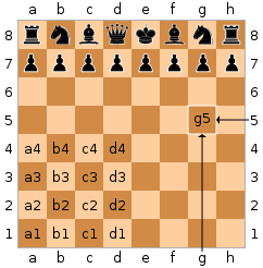
A board state will be a set of qubits that represent a set of squares. We will often consider a board that is smaller than the standard 8x8 board of chess so that we can more easily illustrate concepts.
For instance, let's consider a 3x3 board. This board will have 9 squares (a1, a2, a3, b1, b2, b3, c1, c2, c3). We will represent this as a 'ket' string such as this, with spaces to denote row boundaries for ease of reading:
|a1a2a3 b1b2b3 c1c2c3 >
For instance, |000 000 000> would represent the empty 3x3 board. |010 000 000> would represent a piece on the 'a2' square. States can also represent boards with multiple pieces. |000 000 110> would represent a board with pieces on both 'c1' and 'c2'. Each of these three states is denoted as a basis state.
A state can also be a super-position of board states. For instance,
\(\frac{1}{\sqrt{2} }\) ( |100 000 000> + |010 000 000> ) represents a piece being in superposition of being on 'a1' and 'a2'. This tutorial will often drop the normalization factor such as \(\frac{1}{\sqrt{2} }\) when it doesn't matter to the explanation.
Additional qubits
Note that there are some exceptions that require extra qubits beyond the requirement of one qubit per square. These extra qubits (often called "ancilla" qubits) are needed to store captured pieces and to store extra information, such as whether a path is blocked by a piece. We will ignore these extra ancilla qubits for now in order to keep the tutorial focused.
Quantum Chess Moves
We will be studying a subset of possible quantum chess moves in this tutorial.
We will primarily consider the following moves to implement on the hardware:
Basic jump move
This maneuver will be applied when we wish to apply a standard chess move to a piece. This will be how kings and knights move. In classical chess, we would remove the piece from its original square and then add it to the target square we are moving it to.
For quantum chess, we would like to do an analogous operation that preserves any quantum information. In order to do this, we will swap the two squares. We will do this by performing an iSWAP gate between the two qubits that represent those squares. Note that this operation will also add a phase of i onto the qubits in addition to swapping them, adding a uniquely quantum aspect to the move.
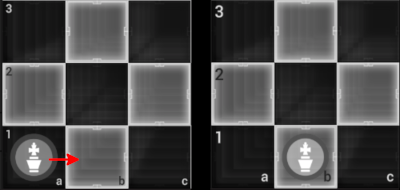
For example, if we attempt to move a King piece from the 'a1' square to the 'b1' square, we will perform a iSWAP gate between the qubits that represent the 'a1' and 'b1' squares.
Split move
The split move is unique to quantum chess. This move will be analogous to moving a piece to two different target squares simultaneously. If we were to then measure the quantum board, we should get a 50% probability of seeing the piece in either of the two target squares.
This will be accomplished by doing a \(\sqrt{\text{iSWAP} }\) between the source and the first target. This will create an equal superposition between the source and the first target square. We would finish the move by performing a iSWAP between the source square and second target square. This will create an equal superposition between the two target squares.
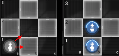
For example, suppose that that we split move a King on 'a1' to the squares 'b1' and 'b2'. To do this, we would do a \(\sqrt{\text{iSWAP} }\) between the qubits representing 'a1' and 'b1' followed by an iSWAP on the 'a1' and 'b2' qubits. A short-hand notation for this move is Ks1^t1t2 for source square s1 and split targets t1 and t2. This example would be noted as Ka1^b1b2.
Slide move
A slide move is how we will move bishops, queens, and rooks. These pieces move along a straight path, but cannot pass through intervening pieces. However, in quantum chess, there may be a piece that is in superposition and may or may not block the path of this move.
In order to accomplish this move without measuring (and thereby destroying the quantum nature of the game), we will need to entangle the two pieces. The way we will do this is called a "controlled" gate. A controlled gate is a gate that is only performed if the control qubit(s) are in the |1> state.
This tutorial will only consider paths that are blocked by one possible piece. In this case, we will perform a controlled-iSWAP between the source square and target square controlled by the square that is potentially blocking the path.
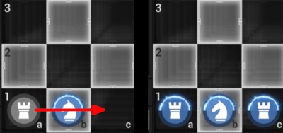
For example, suppose we are moving a rook from 'a1' to 'c1', but there is a split knight on 'b1'. To perform this slide move, we would do an iSWAP between the qubits that represent 'a1' and 'c1' controlled by the 'b1' qubit. This operation can result in two potential states. Either the rook is on 'c1' and the knight is not on 'b1' (path was open) or, alternatively, the rook is on 'a1' and the knight is on 'b1' (path was blocked). The quantum board state cannot be described without mentioning the relationship between the 'b1' and 'a1'/'c1' squares, so we can say that those squares are entangled.
Exclusion move
It was mentioned earlier that each square must have only one type of piece. For instance, a square cannot have 0.1 of a knight and 0.5 of a rook. This would not be allowed. This is called the 'no double occupancy' rule. We will use measurement as a tool to prevent this situation and disambiguate the type of the piece.
This can happen in a variety of circumstances, but we will only consider the case where a piece attempts to make a legal, standard move into a square with a piece of its own color.
For instance, suppose we attempt to move a king from 'a1' to 'a2' and there is a split knight on the 'a2' square. We would then need to measure the 'a2' square. If the measurement is 1, then the knight occupies the square and the king cannot move. If the measurement is 0, the knight is not on the square and the king moves successfully. In this case, we have a classical 'mixture' of states. Half the time, we would get the king on 'a1' and the knight on 'a2'. The other half of the time, the king would be on 'a2'. However, since we have measured and projected the state to one of these possibilities, there would be no superposition or entanglement, and this part of the board would be in a classical state (definitively in either one configuration or the other).
Other moves
These four type of moves are enough to illustrate the complexities of translating an abstract algorithm (quantum chess) onto a concrete hardware implementation. However, those who are curious can see the full rule set in the Quantum Chess paper on arXiv, including for capture, en passant, and castling.
Exercise for the reader: This describes one possible rule set for translating the game of chess into the quantum world. How might the game change if you use SWAP gates instead of iSWAP gates? Can you devise ways to tell the two games apart? Can you think of other methods to create split moves or other interesting alternatives?
Quantum Chess Simulation
Now that we have introduced the moves of quantum chess and their corresponding circuits, let's look at how we might actually perform our quantum chess moves and circuits in hardware. We will first start by learning how to implement them in cirq and how to execute them using cirq's built-in simulator.
If we consider that a chess board has 64 squares, then the simulation will need 64 qubits. Since any combination of these bits is a valid basis state of the system, this means that, in order to do a complete simulation, we will need to keep track of \(2^{64}\) states, which is something around 10 quintillion states. This is obviously infeasible.
However, most of these positions are unreachable by any common set of moves. For most reasonable positions, there is a much smaller amount of superposition, so we do not need to keep track of all of those states, since the probability of those states is zero and will remain zero after we make our moves.
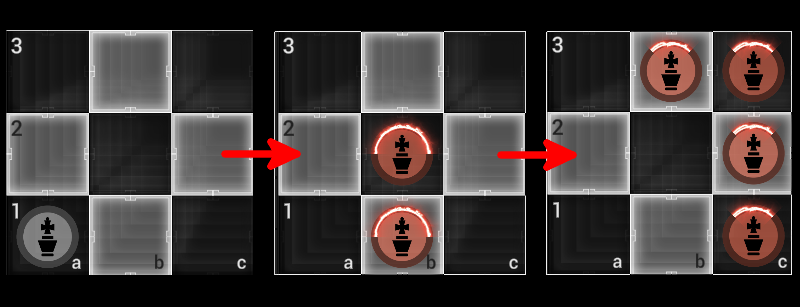
For example, the initial position is a classical position, so we only need to keep track of one possible state, where the initial squares are in the |1> state and the empty squares are in the |0> state. After we make a split move, now we have to keep track of two states. Each successive move on the board will need to tabulate its effect on both of these possible states.
Example:
Let's consider a 3x3 board as defined above with one King piece that starts in the square 'a1'. This initial state is:
|100 000 000>
Note that, since there are 9 squares, there are \(2^9=512\) possible basis states and a position on this board could be a superposition of any of the 512 basis states.
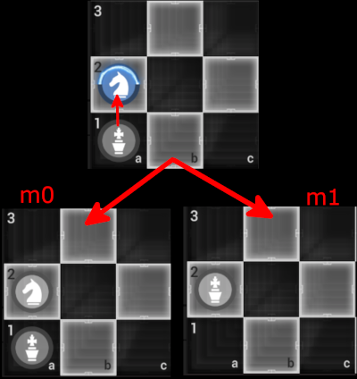
For instance, let's suppose that we now perform a split move from 'a1' to 'b1' and 'b2'. Then the state will be (ignoring the factor of \(i/{\sqrt{2} }\)):
|000 010 000> + |000 100 000>
Now, suppose that we make two additional moves. First, we will split the "half-king" on 'b1' to 'c1' and 'c2'. Next, we will split the 'half king' on 'b2' to 'b3' and 'c3'.
So, despite that we have made three split moves that involve almost all of the squares on the board, we still only have to worry about 4 of the 512 states on the board. The state is now (ignoring the constant factor):
|000 000 100> + |000 000 010> + |000 001 000> + |000 000 001>
Of course, if we continue splitting moves, we will eventually get to a large number of potential states. However, we will never need to consider all 512 states in this example, since some states can never be reached by a sequence of moves. For instance, the state |110 000 000> represents a king on a1 and a king on b1. There's no way where we can start the board with one king on the board and suddenly wind up with two kings (unless we have noise, more on that later).
Exercise to the reader: How many basis states are possible to include in a superposition if we allow the player to make as many normal/split moves as they want? How many superpositions are possible?
Summary
Since the space of possible quantum chess positions is much smaller than the space of possible quantum states, it is very tractable to simulate quantum chess if we have a custom simulator tuned to consider only relevant states.
Quantum Chess in Cirq
Next, let's define each of these moves in cirq. We will define a function for each of three possible moves we are considering. Each of these will use make use of a python structure called generators which allows us to 'yield' one or more operations. This will allow us to use these functions very flexibly while we construct circuits.
In addition, we will define a function for placing a piece on the board. Cirq simulators initialize into the zero state (an empty board), so we will use an 'X' gate to turn on a qubit and place a piece on the board.
def normal_move(s: cirq.Qid, t: cirq.Qid):
    """A normal move in quantum chess.

    This function takes two qubits and returns a generator
    that performs a normal move that moves a piece from the
    source square to the target square.

    Args:
        s: source qubit (square where piece starts)
        t: target qubit (square to move piece to)
    """
    yield cirq.ISWAP(s, t)


def split_move(s: cirq.Qid, t1: cirq.Qid, t2: cirq.Qid):
    """A Split move in quantum chess.

    This function takes three qubits and returns a generator
    that performs a split move from the source qubit to the
    two target qubits.

    Args:
        s: source qubit (square where piece starts)
        t1: target qubit (first square to move piece to)
        t2: target qubit (second square to move piece to)
    """
    yield cirq.ISWAP(s, t1) ** 0.5
    yield cirq.ISWAP(s, t2)


def slide_move(s: cirq.Qid, t: cirq.Qid, p: cirq.Qid):
    """A Slide move in quantum chess.

    This function takes three qubits and returns a generator
    that performs a slide move.  This will move a piece
    from the source to the target controlled by the path qubit.
    The move will only occur if the path qubit is turned on
    (i.e. path qubit should be one if the path is unblocked).

    Args:
        s: source qubit (square where piece starts)
        t: target qubit (square to move piece to)
        p: path qubit that determines whether move should occur
    """
    yield cirq.ISWAP(s, t).controlled_by(p)


def place_piece(s: cirq.Qid):
    """Place a piece on the board.

    This is not actually a move.  However, since qubits in Cirq
    default to starting in the |0> state, we will need to activate
    the qubit by applying an X gate to initialize the position.
    """
    yield cirq.X(s)
Now that the moves are defined as gates in Cirq, let's now define the qubits. Since we haven't figured out how we will represent this on the hardware, we will use Cirq's concept of NamedQubit in order to define the squares as logical qubits without defining a device topology. This may feel unusual to some, but it can be compared to "textbook" circuits that have lines for abstract qubits that are unnamed or have simple symbolic names. We will first try to define our algorithm in the abstract case, then move towards a physical representation at the end of this colab.
a1 = cirq.NamedQubit("a1")
a2 = cirq.NamedQubit("a2")
a3 = cirq.NamedQubit("a3")
b1 = cirq.NamedQubit("b1")
b2 = cirq.NamedQubit("b2")
b3 = cirq.NamedQubit("b3")
c1 = cirq.NamedQubit("c1")
c2 = cirq.NamedQubit("c2")
c3 = cirq.NamedQubit("c3")

all_squares = [a1, a2, a3, b1, b2, b3, c1, c2, c3]
Now that we have a 3x3 'board' of qubits, let's try to perform some moves.
Let's try to create the circuit mentioned in our simulator example that places a king on the 'a1' square, then splits to 'b1' and 'b2', then further splits to 'c1' and 'c2' and then to 'b3' and 'c3'.
king_moves = cirq.Circuit(
    place_piece(a1),
    split_move(a1, b1, b2),
    split_move(b1, c1, c2),
    split_move(b2, b3, c3),
)

# Let's print out the circuit to see what it does
print(king_moves)

# Let's also simulate it using cirq's built-in simulator
sim = cirq.Simulator()
sim.simulate(king_moves)
┌──────────────┐   ┌──────────────┐
a1: ───X───iSwap────────iSwap────────────────────────────────────────
           │            │
b1: ───────iSwap^0.5────┼────iSwap─────────iSwap─────────────────────
                        │    │             │
b2: ────────────────────iSwap┼─────────────┼────iSwap────────iSwap───
                             │             │    │            │
b3: ─────────────────────────┼─────────────┼────iSwap^0.5────┼───────
                             │             │                 │
c1: ─────────────────────────iSwap^0.5─────┼─────────────────┼───────
                                           │                 │
c2: ───────────────────────────────────────iSwap─────────────┼───────
                                                             │
c3: ─────────────────────────────────────────────────────────iSwap───
                       └──────────────┘   └──────────────┘
measurements: (no measurements)

qubits: (cirq.NamedQubit('a1'), cirq.NamedQubit('b1'), cirq.NamedQubit('b2'), cirq.NamedQubit('c1'), cirq.NamedQubit('c2'), cirq.NamedQubit('b3'), cirq.NamedQubit('c3'))
output vector: -0.5|0000001⟩ - 0.5|0000010⟩ - 0.5|0000100⟩ - 0.5|0001000⟩

phase:
output vector: |⟩
Fantastic! We can clearly see that the result from the simulator shows a superposition of 4 states! So far, so good.
Let's try a slightly more complicated example involving two pieces and an exclusion move that forces a measurement.
Let's start with a king on 'a1' and a queen on 'a3'. We will split the king onto 'b1' and 'b2' as before. Next, we will split move the king on 'b1' to 'c1' and 'c2'. Lastly, we will try to move the queen from 'a3' to 'b2'.
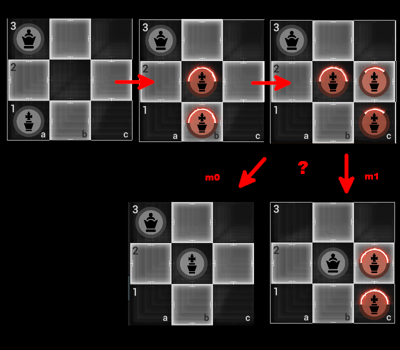
This will trigger a condition known as "double occupancy". We are not allowed to have two pieces of different types in the same square. If the king is in 'b2', the queen cannot move there. If the king is not in 'b2', then the move is legal. Thus, we will need to do a measurement. Let's see how that works.
exclusion_moves = cirq.Circuit(
    place_piece(a1),
    place_piece(a3),
    split_move(a1, b1, b2),
    split_move(b1, c1, c2),
)
exclusion_move_circuit = exclusion_moves + cirq.measure(b2)


# Let's print out the circuit to see what it does
print("Exclusion move circuit:")
print(exclusion_move_circuit)

# This time, we have a measurement in the circuit.
# Let's simulate it several times to see what happens.
sim = cirq.Simulator()
print("Measurement Results:")
for t in range(8):
    print(f"--- Outcome #{t} ---")
    print(sim.simulate(exclusion_move_circuit))
Exclusion move circuit:
                       ┌──────────────┐   ┌──────┐
a1: ───X───iSwap────────iSwap────────────────────────
           │            │
a3: ───X───┼────────────┼────────────────────────────
           │            │
b1: ───────iSwap^0.5────┼────iSwap─────────iSwap─────
                        │    │             │
b2: ────────────────────iSwap┼─────────────┼────M────
                             │             │
c1: ─────────────────────────iSwap^0.5─────┼─────────
                                           │
c2: ───────────────────────────────────────iSwap─────
                       └──────────────┘   └──────┘
Measurement Results:
--- Outcome #0 ---
measurements: b2=0

qubits: (cirq.NamedQubit('a1'), cirq.NamedQubit('b1'), cirq.NamedQubit('c1'), cirq.NamedQubit('c2'))
output vector: 0.707|0001⟩ + 0.707|0010⟩

qubits: (cirq.NamedQubit('a3'),)
output vector: |1⟩

qubits: (cirq.NamedQubit('b2'),)
output vector: -1|0⟩

phase:
output vector: |⟩
--- Outcome #1 ---
measurements: b2=1

qubits: (cirq.NamedQubit('a1'), cirq.NamedQubit('b1'), cirq.NamedQubit('c1'), cirq.NamedQubit('c2'))
output vector: |0000⟩

qubits: (cirq.NamedQubit('a3'),)
output vector: |1⟩

qubits: (cirq.NamedQubit('b2'),)
output vector: 1j|1⟩

phase:
output vector: |⟩
--- Outcome #2 ---
measurements: b2=1

qubits: (cirq.NamedQubit('a1'), cirq.NamedQubit('b1'), cirq.NamedQubit('c1'), cirq.NamedQubit('c2'))
output vector: |0000⟩

qubits: (cirq.NamedQubit('a3'),)
output vector: |1⟩

qubits: (cirq.NamedQubit('b2'),)
output vector: 1j|1⟩

phase:
output vector: |⟩
--- Outcome #3 ---
measurements: b2=1

qubits: (cirq.NamedQubit('a1'), cirq.NamedQubit('b1'), cirq.NamedQubit('c1'), cirq.NamedQubit('c2'))
output vector: |0000⟩

qubits: (cirq.NamedQubit('a3'),)
output vector: |1⟩

qubits: (cirq.NamedQubit('b2'),)
output vector: 1j|1⟩

phase:
output vector: |⟩
--- Outcome #4 ---
measurements: b2=0

qubits: (cirq.NamedQubit('a1'), cirq.NamedQubit('b1'), cirq.NamedQubit('c1'), cirq.NamedQubit('c2'))
output vector: 0.707|0001⟩ + 0.707|0010⟩

qubits: (cirq.NamedQubit('a3'),)
output vector: |1⟩

qubits: (cirq.NamedQubit('b2'),)
output vector: -1|0⟩

phase:
output vector: |⟩
--- Outcome #5 ---
measurements: b2=1

qubits: (cirq.NamedQubit('a1'), cirq.NamedQubit('b1'), cirq.NamedQubit('c1'), cirq.NamedQubit('c2'))
output vector: |0000⟩

qubits: (cirq.NamedQubit('a3'),)
output vector: |1⟩

qubits: (cirq.NamedQubit('b2'),)
output vector: 1j|1⟩

phase:
output vector: |⟩
--- Outcome #6 ---
measurements: b2=0

qubits: (cirq.NamedQubit('a1'), cirq.NamedQubit('b1'), cirq.NamedQubit('c1'), cirq.NamedQubit('c2'))
output vector: 0.707|0001⟩ + 0.707|0010⟩

qubits: (cirq.NamedQubit('a3'),)
output vector: |1⟩

qubits: (cirq.NamedQubit('b2'),)
output vector: -1|0⟩

phase:
output vector: |⟩
--- Outcome #7 ---
measurements: b2=0

qubits: (cirq.NamedQubit('a1'), cirq.NamedQubit('b1'), cirq.NamedQubit('c1'), cirq.NamedQubit('c2'))
output vector: 0.707|0001⟩ + 0.707|0010⟩

qubits: (cirq.NamedQubit('a3'),)
output vector: |1⟩

qubits: (cirq.NamedQubit('b2'),)
output vector: -1|0⟩

phase:
output vector: |⟩
In this configuration, you should see two different results. If we measured the king to be at 'b2', then the position is resolved to a single basis state, equivalent to a classical position (the king is at 'b2' and the queen is at 'a3').
If the 'b2' square is measured to be empty, then the board is still in a state of superposition.
Handling Partial Measurement
So far, we have been simulating this using cirq.simulate() which shows us the waveform of the system and its internal state. In a quantum device, we do not have this information. All we have is the measurement data that we get out of the device. Let's try both of these circuits again with the simulator, but denying ourselves access to the underlying wave function, solely using measurement results.
First, we will need to add measurements to our previous circuits so that we can access statistical data.
# Define a measurement operation that measures all the squares
measure_all_squares = cirq.measure(*all_squares, key="all")

# Measure all squares at the end of the circuit
king_moves_measured = king_moves + measure_all_squares
exclusion_move_measured = exclusion_moves + measure_all_squares

print("Split moving the king:")
print(king_moves_measured)
results = sim.run(king_moves_measured, repetitions=1)
print(results)

print("Attempting an exclusion move:")
results = sim.run(exclusion_move_measured, repetitions=1)
print(results)
Split moving the king:
                       ┌──────────────┐   ┌──────────────┐
a1: ───X───iSwap────────iSwap────────────────────────────────────────M('all')───
           │            │                                            │
a2: ───────┼────────────┼────────────────────────────────────────────M──────────
           │            │                                            │
a3: ───────┼────────────┼────────────────────────────────────────────M──────────
           │            │                                            │
b1: ───────iSwap^0.5────┼────iSwap─────────iSwap─────────────────────M──────────
                        │    │             │                         │
b2: ────────────────────iSwap┼─────────────┼────iSwap────────iSwap───M──────────
                             │             │    │            │       │
b3: ─────────────────────────┼─────────────┼────iSwap^0.5────┼───────M──────────
                             │             │                 │       │
c1: ─────────────────────────iSwap^0.5─────┼─────────────────┼───────M──────────
                                           │                 │       │
c2: ───────────────────────────────────────iSwap─────────────┼───────M──────────
                                                             │       │
c3: ─────────────────────────────────────────────────────────iSwap───M──────────
                       └──────────────┘   └──────────────┘
all=0, 0, 0, 0, 0, 1, 0, 0, 0
Attempting an exclusion move:
all=0, 0, 1, 0, 1, 0, 0, 0, 0
You'll notice that, if you run the above block multiple times, you will get different results.
We will need a way to compile these into a statistical measure. For this, we will need to increase the number of repetitions, and then combine them into a histogram. Let's write a simple function to aggregate the results from the simulator (which are returned in a numpy array) into a more convenient form for us.
def histogram_of_squares(results):
    """Creates a histogram of measurement results per square.

    Returns:
        Dict[str, int] where the key is the name of the square and the
        value is the number of times the square was measured in the one state.
    """
    sampling_frequency = {}
    for idx, sq in enumerate(all_squares):
        sampling_frequency[str(sq)] = results.measurements["all"][:, idx].sum()
    return sampling_frequency


# Let's test out this histogram on the two circuits we've examined so far:

print("Split moving the king:")
split_results = sim.run(king_moves_measured, repetitions=1000)
print(histogram_of_squares(split_results))

print("Attempting an exclusion move:")
exclusion_results = sim.run(exclusion_move_measured, repetitions=1000)
print(histogram_of_squares(exclusion_results))
Split moving the king:
{'a1': 0, 'a2': 0, 'a3': 0, 'b1': 0, 'b2': 0, 'b3': 272, 'c1': 234, 'c2': 251, 'c3': 243}
Attempting an exclusion move:
{'a1': 0, 'a2': 0, 'a3': 1000, 'b1': 0, 'b2': 514, 'b3': 0, 'c1': 243, 'c2': 243, 'c3': 0}
We can now see the frequencies of different possibilities. For our first situation, we can see the king has four possibilities with approximately the same amount of occurrences. Due to statistical variations, the exact number of occurrences in each of the four squares is not exactly the same.
Our second exclusion move example illustrates the king's possible position on the three different squares, but we have not yet figured out how to implement the queen's exclusion and measurement with the king.
How are we going to do that?
First, we need to pick a sample that will become our official "measurement" for the board. We will freeze the seed for the random number generator so that everyone running this colab gets the same measurement and measure the square we care about (b2).
exclusion_move_measure_b2 = exclusion_moves + cirq.measure(b2)

this_sim = cirq.Simulator(seed=1234)
measurement_for_move = this_sim.run(exclusion_move_measure_b2, repetitions=1)
print(measurement_for_move)
b2=0
When we measure the square 'b2', it is empty. (The above should consistently print out 'b2=0'. If it doesn't, you can change your seed so it does). Thus, we can now move the queen.
Ok, we are now ready to make the next move. How do we figure out the statistics of the board and be able to compute the (quantum) state of the board so that we can continue the game?
Let's try to move the queen and see what happens:
# Calculate the state of the board after moving the queen
after_exclusion_move = (
    cirq.Circuit(
        place_piece(a1),
        place_piece(a3),
        split_move(a1, b1, b2),
        split_move(b1, c1, c2),
        normal_move(a3, b2),
    )
    + measure_all_squares
)

# Compute statistics for the pieces.
after_results = this_sim.run(after_exclusion_move, repetitions=1000)
print(histogram_of_squares(after_results))
{'a1': 0, 'a2': 0, 'a3': 484, 'b1': 0, 'b2': 1000, 'b3': 0, 'c1': 227, 'c2': 289, 'c3': 0}
Uh oh. This is not correct. The queen now has 100% probability of being on 'b2', but there is now a king at 'a3' with approximately 50% probability.
The problem is that we are including both the possibility that the king was at 'b2' as well as the possibility that it was empty. Instead of initializing the king to 'a1', we could initialize the king to 'b1' and just do one split move from 'b1' to 'c1' and 'c2' instead of performing all operations since the beginning of the game.
This has two issues. First is that we are cheating somewhat by using the simplicity of this toy example to only include paths that are possible. In a more complicated game, with pieces and merges happening, it may be a lot more difficult to simplify the circuit in a way that replicates the results of a measurement. The second problem is that we have discarded information about the relative phases of the pieces. For instance, the different squares could have picked up phases of \(i\), and we would not be able to tell by just looking at the measurement results. We may be destroying this information by simplifying the circuit.
Exercise to the reader: Is the phase actually the same or different if we compute the shorter circuit?
So then, how do we handle this?
Post-selection
One way of resolving this is to use the method of "post-selection". Both simulators and real hardware have the ability to repeat an experiment many times. We can use this ability to pick the samples that match our expectations of the results.
In the example above, we have two independent possibilities for the measurement of the king. Half of results will have 'm0' (the king was on the square preventing the queen move) and half will have 'm1' result (the king was not there and the queen move was possible). In our game, we know that 'm1' is what happened, so we can run the simulation multiple times and only take the results that are consistent with 'm1'.
This procedure is only needed since we need to run the simulation from the beginning of the board each time. If we could "save" the state vector from the last move, we would not need to do this. We could just apply the next move on the last state vector. While this is possible in a classical simulator, quantum states in a real device only stay coherent for mere microseconds and won't wait around while we ponder our next quantum chess move.
A quantum algorithm that uses results of measurements to affect later steps is called a "feed-forward". We are going to use post-selection to transform the current feed-forward algorithm of quantum chess into an algorithm that has terminal measurements only.
We will transform our first algorithm from:
- Make some non-measurement moves.
- Make a move that requires measurement and gets an outcome of 'm1'
- Make a second set of non-measurement moves based on this outcome.
Into the following new algorithm:
- Make some non-measurement moves.
- Make the exclusion move but don't measure yet.
- Make the second set of moves.
- Measure the relevant qubits. Discard results that do not match our expected result of 'm1'
Note that we have to be careful when we do this. First, we have to track the qubits to perform the correct measurement. In our example above, the queen moved to the 'b2' square, regardless of whether the king was there. Executing that move swapped the qubits of 'b2' and 'a3'. So, when we measure the king's position at the end of the circuit, we need to measure its new position within the 'a3' qubit.
Second, we need to ensure that the two outcomes are truly independent. If further moves begin interacting with our 'a3' square that holds the position of the king, then we may get incorrect results. To do this correctly, we may want to swap the king's state into an ancillary qubit so that it doesn't interact with further moves. This is left as an exercise to the reader.
The following code shows how we might do this for the example circuit:
# Perform all the moves, including the exclusion move.
# Afterwards, measure all qubits.
after_exclusion_move = (
    cirq.Circuit(
        place_piece(a1),
        place_piece(a3),
        split_move(a1, b1, b2),
        split_move(b1, c1, c2),
        normal_move(a3, b2),
    )
    + measure_all_squares
)

# Define a function to post select on the result.
def histogram_post_select(results, square_idx, value):
    """Return a histogram of measurement results with post-selection.

    This will return a dictionary of str to int, with the key being
    the name of the square and the value being the number of times the
    square was measured as one. These results will exclude any results
    where the square represented by `square_idx` were not equal to `value`.

    Args:
        results: TrialResults returned by a sampler.
        square_idx: integer index of the measured qubit to post-select on.
        value: whether the qubit post-selected should be one or zero.
    """
    sampling_frequency = {}
    all_results = results.measurements["all"]
    post_selected_results = all_results[all_results[:, square_idx] == value]
    for idx, sq in enumerate(all_squares):
        sampling_frequency[str(sq)] = post_selected_results[:, idx].sum()
    return sampling_frequency


# Compute statistics for the pieces.
after_results = this_sim.run(after_exclusion_move, repetitions=1000)

# Find the index of 'a3' (it should be at index 2)
post_select_idx = all_squares.index(cirq.NamedQubit("a3"))

# Print out the post-selected histogram
print(histogram_post_select(after_results, post_select_idx, 0))
{'a1': 0, 'a2': 0, 'a3': 0, 'b1': 0, 'b2': 503, 'b3': 0, 'c1': 246, 'c2': 257, 'c3': 0}
We now have about half the number of results, but they only include results with the relevant measurement outcomes. We now have replicated the correct state of the board after the exclusion board.
To show that we can use this state to continue the quantum chess game, let's make a final move from the king from c2 to c3. This represents the board state with king on 'a1', queen on 'a3' after the moves Ka1^b1b2, Kb1^c1c2, Qa3b2.m1, Kc2c3:
after_exclusion_without_measurement = cirq.Circuit(
    place_piece(a1),
    place_piece(a3),
    split_move(a1, b1, b2),
    split_move(b1, c1, c2),
    normal_move(a3, b2),
    normal_move(c2, c3),
)
after_exclusion_move = (
    after_exclusion_without_measurement + measure_all_squares
)

after_results = this_sim.run(after_exclusion_move, repetitions=1000)
post_select_idx = all_squares.index(cirq.NamedQubit("a3"))
print(histogram_post_select(after_results, post_select_idx, 0))
{'a1': 0, 'a2': 0, 'a3': 0, 'b1': 0, 'b2': 507, 'b3': 0, 'c1': 242, 'c2': 0, 'c3': 265}
We can now see that the measurements that were on 'c2' have now moved to 'c3'. This illustrates how we can continue a quantum chess move sequence that contains a partial measurement part-way through the sequence, even on a device that only supports final measurement!
Noise
So far, we have dealt with a simulator that is completely noiseless. Even so, we have already seen statistical fluctuations that affect our probabilities. Real NISQ devices will have a lot of noise that will affect calculations in every way possible.
There are many components to noise. Some possible (overlapping) sources of noise include:
- T1 Decay / relaxation: Qubits in the excited state \(\vert 1\rangle\) could lose energy and fall into the ground state \(\vert 0\rangle\). This is typically qualified by a metric called T1 that specifies the rate of exponential decay (similar to a "half-life" of radioactive decay).
- Dephasing error: Qubits could be "spinning" in relation to each other. For instance, a qubit in \(\frac{1}{\sqrt{2} } (\vert0\rangle + \vert 1\rangle)\) could become \(\frac{1}{\sqrt{2} } (\vert0\rangle + i\vert 1\rangle)\). This is sometimes simplified to a measure called T2 or T2*. However, since dephasing errors can "spin" at many different rates and directions, a full noise spectrum is needed to fully characterize these types of errors.
- Readout/measurement error: If we accidentally detect a \(\vert 0\rangle\) as a \(\vert 1\rangle\) or vice versa when performing a measurement, this is often classified as a readout error.
- Control/Coherent error: The device can drift out of calibration or can be too difficult to control effectively. If every time that we do a \(\text{iSWAP}\) gate, we consistently do a \(\text{iSWAP}^{0.98}\), this is a coherent error.
- Cross talk: Effects that involve specific pairs of (usually nearby) qubits could occur that can create correlations or entanglements. These effects are often more difficult to model and fix.
Luckily, we don't need an actual hardware device to simulate (some of these) noisy effects. We can simulate them using cirq's simulator.
Let's run the simulator with the moves Ka1^b1b2, Kb1^c1c2, Kb2^b3c3 that we were examining before, but this time using one of cirq's noise models called a depolarizing channel that randomly scrambles a qubit with a set probability.
import cirq.contrib.noise_models as ccn

noise_model = ccn.DepolarizingNoiseModel(depol_prob=0.01)
noisy = cirq.DensityMatrixSimulator(noise=noise_model)

king_moves_measured = (
    cirq.Circuit(
        place_piece(a1),
        split_move(a1, b1, b2),
        split_move(b1, c1, c2),
        split_move(b2, b3, c3),
    )
    + measure_all_squares
)

print(histogram_of_squares(noisy.run(king_moves_measured, repetitions=1000)))
{'a1': 30, 'a2': 0, 'a3': 0, 'b1': 33, 'b2': 44, 'b3': 272, 'c1': 291, 'c2': 261, 'c3': 253}
These results look a lot messier than what we were looking at before. First, all 9 squares have some probability of the king being there, even though there is no possibility that the king can be there. That's a problem.
Also, the results no longer add up to 1000. Uh oh. How is that even possible? Have we made a mistake?
If noise flips some of the qubits to |1>, we can now measure a state that records the king in two places. For instance |100 000 001> is a state that could be achieved with a single incorrect bit flip and represents the board state with two kings: one on 'a1' and one on 'c3'. This will give us two entries in the histogram for a single repetition of the circuit, causing the total to exceed 1000.
We know that there is no way to create pieces in chess, so some of these results are nonsensical.
One way to do error mitigation is to detect these nonsensical events and remove them. Let's recode this to use "post-selection" to exclude measurements that have more than one king (or that have zero kings), which we know are impossible positions to reach in this situation.
def remove_multi_kings(results):
    """Removes samples from a set of results that do not have one measurement.

    Returns a histogram dictionary as defined above that only has results that
    have one square with a measurement outcome of one and all other squares have
    measurement outcomes of zero.  Results that do not fit this pattern are
    discarded.
    """
    sampling_frequency = {}
    all_results = results.measurements["all"]
    # Select only rows where the row sums to one.
    post_selected_results = all_results[all_results[:, :].sum(axis=1) == 1]
    for idx, sq in enumerate(all_squares):
        sampling_frequency[str(sq)] = post_selected_results[:, idx].sum()
    return sampling_frequency


results = noisy.run(king_moves_measured, repetitions=1000)
print(remove_multi_kings(results))
{'a1': 2, 'a2': 0, 'a3': 0, 'b1': 2, 'b2': 1, 'b3': 190, 'c1': 223, 'c2': 196, 'c3': 201}
This data is much better! We have not eliminated all the noise, but, by taking into account the constraints and invariants of the problem we are trying to solve, we have eliminated much of the noise!
Next, let's look at another source of noise.
Coherent noise
Let's say that our device consistently performs incorrect operations, but that we do not know the exact nature of these errors. Is there a way to correct for these types of problems?
Let's suppose that, instead of doing an iSWAP, our device does part of an iSWAP, but that amount differs from day to day and we don't know what the percentage of an iswap is going to be. One day it could be 50% of an iSWAP, and the next day it could be 80% of an iSWAP. We don't know what that percentage is, but we know that it will stay fairly stable throughout our calculation.
How would that affect our results? Let's define a function called "lazy_move" that represents this partial iSWAP. Then, let's march the king from a1 to a2 to a3 to b3 to c3 using this under-rotated iSWAP and see what happens.
import random

# Define our secret under-rotation parameter once across multiple executions.
try:
    _secret_lazy_value
except:
    _secret_lazy_value = (random.random() + 2.0) / 4.0


def lazy_move(source, target):
    return cirq.ISWAP(source, target) ** _secret_lazy_value


king_maybe_moves = (
    cirq.Circuit(
        place_piece(a1),
        lazy_move(a1, a2),
        lazy_move(a2, a3),
        lazy_move(a3, b3),
        lazy_move(b3, c3),
    )
    + measure_all_squares
)

print(histogram_of_squares(sim.run(king_maybe_moves, repetitions=1000)))
{'a1': 213, 'a2': 148, 'a3': 124, 'b1': 0, 'b2': 0, 'b3': 92, 'c1': 0, 'c2': 0, 'c3': 423}
As we run this circuit, we see that the king leaks across the path it takes and only some of the probability makes it to the final destination. However, this probability remains roughly the same across multiple invocations.
Can we correct or "calibrate" this broken gate so that it is fixed for our use case?
Let's suppose our device supports a rotation angle for our iSWAP gate. Can we over-rotate the gate on purpose to counter-act the device's error?
Let's try it.
over_rotation_amount = 1.46

king_probably_moves = (
    cirq.Circuit(
        place_piece(a1),
        lazy_move(a1, a2) ** over_rotation_amount,
        lazy_move(a2, a3) ** over_rotation_amount,
        lazy_move(a3, b3) ** over_rotation_amount,
        lazy_move(b3, c3) ** over_rotation_amount,
    )
    + measure_all_squares
)

print(histogram_of_squares(sim.run(king_probably_moves, repetitions=1000)))
{'a1': 4, 'a2': 0, 'a3': 1, 'b1': 0, 'b2': 0, 'b3': 5, 'c1': 0, 'c2': 0, 'c3': 990}
This looks better, but still not perfect.
In a real example, you may need to tune the operations slightly automatically to correct for coherent error. This is vastly simplified example of what is being performed when a quantum device is being calibrated. The device operator is attempting to perfect the physical operations (such as microwave pulses) to match the intended logical operation (such as iSWAP). Even as a user of a calibrated device, sometimes procedures like this are needed since the operations may not be uniform across the entire processor, and they may drift over time.
Let's write a routine to try to optimize our over rotation constant in order to automatically tune out the under-rotation. In this example, we will do a linear sweep using a parameter value to find the best value. In a real example, you may want to use a gradient optimizer such as scipy.
import sympy

# Our calibration will be to perform one swap
# We will then measure how many times the king actually gets there.
king_calibration = cirq.Circuit(
    place_piece(a1),
    lazy_move(a1, a2) ** sympy.Symbol("r"),
    cirq.measure(a1, a2, key="all"),
)

# We will try all rotation values from 1.0 to 3.0 at intervals of 0.01
rotation_parameter = cirq.Linspace("r", 1.0, 3.0, 200)
results = sim.run_sweep(
    king_calibration, params=rotation_parameter, repetitions=1000
)

# Then we will keep track of the best value we found so far.
best_over_rotation = 1.0
most_correct_swaps = 0
for result in results:
    num_correct_swaps = result.measurements["all"][:, 1].sum()
    if num_correct_swaps > most_correct_swaps:
        most_correct_swaps = num_correct_swaps
        best_over_rotation = result.params["r"]

print(f"Best over rotation value found: {best_over_rotation}")
print(f"Implied secret swap value: {1/best_over_rotation}")
print(f"Actual secret swap value: {_secret_lazy_value}")
Best over rotation value found: 1.4020100502512562
Implied secret swap value: 0.7132616487455198
Actual secret swap value: 0.7082684073833525
Our calibration found a rotation value that corrects for the under-rotation.
Exercise to the reader: Is there a way to get closer to the correct result? Hint: it may cause the simulation to take longer to run.
There are many other types of noise, but it is inevitable that you will need to think about noise as you develop your own applications and mitigate the error to the largest extent possible if you want your application to be successful.
Decomposition
Most devices in the NISQ era will only support certain gate types, often referred to as a gate set.
Let's suppose that our device only supports one two-qubit gate, the \(\sqrt{\text{iSWAP} }\) gate cirq.ISWAP ** 0.5.
How does that affect our quantum chess circuits?
Luckily, most of the moves use either \(\sqrt{\text{iSWAP} }\) gates or \(\text{iSWAP}\) gates (which are merely two \(\sqrt{\text{iSWAP} }\) gates in a row).
However, the slide move (which we have ignored so far), is a \(\text{controlled-iSWAP}\) gate. How will we perform this on hardware?
We will need to transform it into gates we understand. This is often called "decomposing" the gate.
First, let's explore some of cirq's capability in this area. Cirq has some decomposition routines for known gates. Let's see what happens when we decompose the Hadamard \(\text{H}\) gate and the two-qubit \(\text{CNOT}\) gate.
print("Decomposing H gate")
decomposed_h = cirq.decompose_once(cirq.H(a1))
print(decomposed_h)
print(cirq.Circuit(decomposed_h))
print()

print("Decomposing CNOT gate")
decomposed_cnot = cirq.decompose_once(cirq.CNOT(a1, a2))
print(decomposed_cnot)
print(cirq.Circuit(decomposed_cnot))
print()
Decomposing H gate
[(cirq.Y**0.5).on(cirq.NamedQubit('a1')), cirq.XPowGate(global_shift=-0.25).on(cirq.NamedQubit('a1'))]
a1: ───Y^0.5───X───

Decomposing CNOT gate
[(cirq.Y**-0.5).on(cirq.NamedQubit('a2')), cirq.CZ(cirq.NamedQubit('a1'), cirq.NamedQubit('a2')), (cirq.Y**0.5).on(cirq.NamedQubit('a2'))]
a1: ────────────@───────────
                │
a2: ───Y^-0.5───@───Y^0.5───
cirq decomposes an H into a Y rotation and then a X rotation. It decomposes a \(\text{CNOT}\) into a \(\text{CZ}\) gate with some single-qubit gates. Neat, but it doesn't help us get closer to our goal of decomposing to a \(\sqrt{\text{iSWAP} }\).
Let's see what happens when we decompose the \(\text{controlled-iSWAP}\) gate.
cirq.decompose_once(cirq.ISWAP(a1, a3).controlled_by(a2))
[cirq.TOFFOLI(cirq.NamedQubit('a2'), cirq.NamedQubit('a1'), cirq.NamedQubit('a3')),
 cirq.H(cirq.NamedQubit('a1')).controlled_by(cirq.NamedQubit('a2')),
 cirq.TOFFOLI(cirq.NamedQubit('a2'), cirq.NamedQubit('a3'), cirq.NamedQubit('a1')),
 (cirq.CZ**0.5).on(cirq.NamedQubit('a2'), cirq.NamedQubit('a1')),
 cirq.TOFFOLI(cirq.NamedQubit('a2'), cirq.NamedQubit('a3'), cirq.NamedQubit('a1')),
 (cirq.CZ**-0.5).on(cirq.NamedQubit('a2'), cirq.NamedQubit('a1')),
 cirq.H(cirq.NamedQubit('a1')).controlled_by(cirq.NamedQubit('a2')),
 cirq.TOFFOLI(cirq.NamedQubit('a2'), cirq.NamedQubit('a1'), cirq.NamedQubit('a3'))]
Oh, yikes. cirq is able to handle decomposing this, but it uses the decomposition of iSWAP with the control bit attached to all gates. The result is an expansion into several three qubit gates and two qubit gates. While correct, this looks to be going the wrong direction in terms of circuit complexity.
We will need a more powerful tool. Let's use the concept of an optimizer. This is a cirq tool that can run through a circuit, making changes as it goes along. It can be used for compiling to a specific gate set, compressing circuits into less space, or other useful transformations.
Luckily, one already exists for compiling to \(\sqrt{\text{iSWAP} }\). cirq.optimize_for_target_gateset. Let's first demonstrate this with the CNOT gate:
print(cirq.optimize_for_target_gateset(cirq.Circuit(cirq.CNOT(a1, a2)), gateset=cirq.SqrtIswapTargetGateset()))
a1: ───PhXZ(a=-0.25,x=0.5,z=0.25)──────iSwap───────PhXZ(a=-0.5,x=1,z=0)───iSwap───────PhXZ(a=-1,x=0.5,z=0.25)─────
                                       │                                  │
a2: ───PhXZ(a=8.22e-09,x=0.75,z=0.5)───iSwap^0.5──────────────────────────iSwap^0.5───PhXZ(a=0.5,x=0.75,z=-0.5)───
Now we can see that, instead of decomposing into a CZ gate, it decomposes the CNOT into \(\sqrt{\text{iSWAP} }\) gates in addition to some one-qubit phased XZ gates.
Let's try it with the more complicated case of a controlled-iSWAP:
c_iswap = cirq.Circuit(cirq.ISWAP(a1, a3).controlled_by(a2))
try:
    cirq.optimize_for_target_gateset(c_iswap, gateset=cirq.SqrtIswapTargetGateset())
except Exception as e:
    print("An error occurred while attempting to optimize: ")
    print(e)
Yuck. It looks like it gets stuck. We will need to help it out a bit to get it into a form that it can understand.
One common transformation that might help is that a controlled-SWAP (often called a Fredkin gate) does have a known transformation into a Toffoli (another three qubit gate that is a controlled-CNOT) and two CNOT gates. Let's double-check that.
import numpy as np

c_swap = cirq.Circuit(cirq.SWAP(a1, a3).controlled_by(a2))
c_swap_decomposed = cirq.Circuit(
    cirq.CNOT(a1, a3), cirq.TOFFOLI(a2, a3, a1), cirq.CNOT(a1, a3)
)
c_swap_unitary = cirq.unitary(c_swap)
c_swap_decomposed_unitary = cirq.unitary(c_swap_decomposed)

print("Unitary of controlled SWAP")
print(c_swap_unitary)
print("Unitary of decomposed circuit")
print(c_swap_decomposed_unitary)
print("Are they equal?")
print(np.isclose(c_swap_unitary, c_swap_decomposed_unitary).all())
Unitary of controlled SWAP
[[1.+0.j 0.+0.j 0.+0.j 0.+0.j 0.+0.j 0.+0.j 0.+0.j 0.+0.j]
 [0.+0.j 1.+0.j 0.+0.j 0.+0.j 0.+0.j 0.+0.j 0.+0.j 0.+0.j]
 [0.+0.j 0.+0.j 1.+0.j 0.+0.j 0.+0.j 0.+0.j 0.+0.j 0.+0.j]
 [0.+0.j 0.+0.j 0.+0.j 0.+0.j 0.+0.j 0.+0.j 1.+0.j 0.+0.j]
 [0.+0.j 0.+0.j 0.+0.j 0.+0.j 1.+0.j 0.+0.j 0.+0.j 0.+0.j]
 [0.+0.j 0.+0.j 0.+0.j 0.+0.j 0.+0.j 1.+0.j 0.+0.j 0.+0.j]
 [0.+0.j 0.+0.j 0.+0.j 1.+0.j 0.+0.j 0.+0.j 0.+0.j 0.+0.j]
 [0.+0.j 0.+0.j 0.+0.j 0.+0.j 0.+0.j 0.+0.j 0.+0.j 1.+0.j]]
Unitary of decomposed circuit
[[1.+0.j 0.+0.j 0.+0.j 0.+0.j 0.+0.j 0.+0.j 0.+0.j 0.+0.j]
 [0.+0.j 1.+0.j 0.+0.j 0.+0.j 0.+0.j 0.+0.j 0.+0.j 0.+0.j]
 [0.+0.j 0.+0.j 1.+0.j 0.+0.j 0.+0.j 0.+0.j 0.+0.j 0.+0.j]
 [0.+0.j 0.+0.j 0.+0.j 0.+0.j 0.+0.j 0.+0.j 1.+0.j 0.+0.j]
 [0.+0.j 0.+0.j 0.+0.j 0.+0.j 1.+0.j 0.+0.j 0.+0.j 0.+0.j]
 [0.+0.j 0.+0.j 0.+0.j 0.+0.j 0.+0.j 1.+0.j 0.+0.j 0.+0.j]
 [0.+0.j 0.+0.j 0.+0.j 1.+0.j 0.+0.j 0.+0.j 0.+0.j 0.+0.j]
 [0.+0.j 0.+0.j 0.+0.j 0.+0.j 0.+0.j 0.+0.j 0.+0.j 1.+0.j]]
Are they equal?
True
With some leaps of intuition or mathematics, one might try to add an operation to the circuit to rotate the swap slightly to get an iSWAP.
Let's add a CZ ** 0.5 gate in the middle to try to change this from a SWAP to an iSWAP.
import numpy as np

c_iswap = cirq.Circuit(cirq.ISWAP(a3, a2).controlled_by(a1))
c_iswap_decomposed = cirq.Circuit(
    cirq.CNOT(a3, a2),
    cirq.TOFFOLI(a1, a2, a3),
    cirq.CZ(a1, a2) ** 0.5,
    cirq.CNOT(a3, a2),
)
c_iswap_unitary = cirq.unitary(c_iswap)
c_iswap_decomposed_unitary = cirq.unitary(c_iswap_decomposed)

print("Unitary of controlled iSWAP")
print(c_iswap_unitary)
print("Unitary of decomposed circuit")
print(c_iswap_decomposed_unitary)
print("Are they equal?")
print(np.isclose(c_iswap_unitary, c_iswap_decomposed_unitary).all())
Unitary of controlled iSWAP
[[1.+0.j 0.+0.j 0.+0.j 0.+0.j 0.+0.j 0.+0.j 0.+0.j 0.+0.j]
 [0.+0.j 1.+0.j 0.+0.j 0.+0.j 0.+0.j 0.+0.j 0.+0.j 0.+0.j]
 [0.+0.j 0.+0.j 1.+0.j 0.+0.j 0.+0.j 0.+0.j 0.+0.j 0.+0.j]
 [0.+0.j 0.+0.j 0.+0.j 1.+0.j 0.+0.j 0.+0.j 0.+0.j 0.+0.j]
 [0.+0.j 0.+0.j 0.+0.j 0.+0.j 1.+0.j 0.+0.j 0.+0.j 0.+0.j]
 [0.+0.j 0.+0.j 0.+0.j 0.+0.j 0.+0.j 0.+0.j 0.+1.j 0.+0.j]
 [0.+0.j 0.+0.j 0.+0.j 0.+0.j 0.+0.j 0.+1.j 0.+0.j 0.+0.j]
 [0.+0.j 0.+0.j 0.+0.j 0.+0.j 0.+0.j 0.+0.j 0.+0.j 1.+0.j]]
Unitary of decomposed circuit
[[1.+0.j 0.+0.j 0.+0.j 0.+0.j 0.+0.j 0.+0.j 0.+0.j 0.+0.j]
 [0.+0.j 1.+0.j 0.+0.j 0.+0.j 0.+0.j 0.+0.j 0.+0.j 0.+0.j]
 [0.+0.j 0.+0.j 1.+0.j 0.+0.j 0.+0.j 0.+0.j 0.+0.j 0.+0.j]
 [0.+0.j 0.+0.j 0.+0.j 1.+0.j 0.+0.j 0.+0.j 0.+0.j 0.+0.j]
 [0.+0.j 0.+0.j 0.+0.j 0.+0.j 1.+0.j 0.+0.j 0.+0.j 0.+0.j]
 [0.+0.j 0.+0.j 0.+0.j 0.+0.j 0.+0.j 0.+0.j 0.+1.j 0.+0.j]
 [0.+0.j 0.+0.j 0.+0.j 0.+0.j 0.+0.j 0.+1.j 0.+0.j 0.+0.j]
 [0.+0.j 0.+0.j 0.+0.j 0.+0.j 0.+0.j 0.+0.j 0.+0.j 1.+0.j]]
Are they equal?
True
This is great. Let's see if we can decompose this circuit using the built-in operations from cirq.
decomposed_circuit = cirq.optimize_for_target_gateset(
    c_iswap_decomposed, gateset=cirq.SqrtIswapTargetGateset()
)
print(f"Circuit: {len(decomposed_circuit)} moments")
print(decomposed_circuit)
Circuit: 45 moments
a1: ─────────────────────────────────────────────────────────────────────────────────PhXZ(a=0.5,x=0.5,z=0.5)──────────iSwap───────PhXZ(a=-0.5,x=1,z=0)───iSwap───────PhXZ(a=0,x=0.5,z=0.25)────────────────────────────────────────────────────────PhXZ(a=-0.25,x=0.5,z=0.25)──────────iSwap───────PhXZ(a=-0.5,x=1,z=0)───iSwap───────PhXZ(a=-1,x=0.5,z=0.25)─────────────────────────────────────────────────────────PhXZ(a=-0.25,x=0.5,z=0.25)───iSwap───────PhXZ(a=-0.5,x=1,z=0)───iSwap───────PhXZ(a=-1,x=0.5,z=0.25)─────────────────────────────────────────────────────────PhXZ(a=-0.25,x=0.5,z=0.25)───iSwap───────PhXZ(a=-0.5,x=1,z=0)───iSwap───────PhXZ(a=-1,x=0.5,z=0.25)──────────────────────────────────────────────────────────PhXZ(a=0.498,x=0.5,z=-0.498)─────iSwap────────────────────────────────────────iSwap───────PhXZ(a=-1,x=0.5,z=0.748)──────────────────────────────────────────────────────────────────────────────────
                                                                                                                      │                                  │                                                                                                                             │                                  │                                                                                                                        │                                  │                                                                                                                        │                                  │                                                                                                                             │                                            │
a2: ───PhXZ(a=2.22e-16,x=0.12,z=0.5)───iSwap───────PhXZ(a=0.5,x=1,z=0)───iSwap───────PhXZ(a=0.112,x=0.729,z=-0.274)───iSwap^0.5──────────────────────────iSwap^0.5───PhXZ(a=1.19e-08,x=0.5,z=1.0)───iSwap───────PhXZ(a=-0.5,x=1,z=0)───iSwap───────PhXZ(a=-0.196,x=0.667,z=1.29e-08)───iSwap^0.5──────────────────────────iSwap^0.5───PhXZ(a=-1.0,x=0.5,z=-0.75)───────iSwap───────PhXZ(a=-0.5,x=1,z=0)───iSwap───────PhXZ(a=1.0,x=0.75,z=0.5)─────iSwap^0.5──────────────────────────iSwap^0.5───PhXZ(a=-1.0,x=0.5,z=-0.75)───────iSwap───────PhXZ(a=-0.5,x=1,z=0)───iSwap───────PhXZ(a=1.0,x=0.75,z=0.5)─────iSwap^0.5──────────────────────────iSwap^0.5───PhXZ(a=-0.196,x=0.667,z=1.0)──────iSwap───────PhXZ(a=-0.5,x=1,z=0)───iSwap───────PhXZ(a=-0.108,x=0.416,z=-0.19)───iSwap^0.5───PhXZ(a=2.22e-16,x=0.364,z=1.0)───iSwap^0.5───PhXZ(a=-0.838,x=0.636,z=0.43)───iSwap───────PhXZ(a=0.5,x=1,z=0)───iSwap───────PhXZ(a=0.5,x=0.25,z=-0.5)───
                                       │                                 │                                                                                                                          │                                  │                                                                                                                               │                                  │                                                                                                                        │                                  │                                                                                                                         │                                  │                                                                                                                                     │                                 │
a3: ───PhXZ(a=0.76,x=0.5,z=-0.76)──────iSwap^0.5─────────────────────────iSwap^0.5───PhXZ(a=-0.5,x=0.76,z=0.75)──────────────────────────────────────────────────────PhXZ(a=1.0,x=0.5,z=0.5)────────iSwap^0.5──────────────────────────iSwap^0.5───PhXZ(a=-0.623,x=1.55e-08,z=-0.25)──────────────────────────────────────────────────PhXZ(a=-5.81e-09,x=0.5,z=-0.5)───iSwap^0.5──────────────────────────iSwap^0.5───PhXZ(a=-0.375,x=1,z=0)──────────────────────────────────────────────────────PhXZ(a=-5.81e-09,x=0.5,z=-0.5)───iSwap^0.5──────────────────────────iSwap^0.5───PhXZ(a=-0.375,x=1,z=0)──────────────────────────────────────────────────────PhXZ(a=-8.22e-09,x=0.25,z=-0.5)───iSwap^0.5──────────────────────────iSwap^0.5───PhXZ(a=-1,x=0.5,z=-0.25)──────────────────────────────────────────────────────────────────PhXZ(a=-0.75,x=0.5,z=0.75)──────iSwap^0.5─────────────────────────iSwap^0.5───PhXZ(a=-1,x=0.5,z=0.75)─────
So, a bit of good news and a bit of bad news. We are able to create a circuit that can run on hardware that only supports \(\sqrt{\text{iSWAP} }\) and single-qubit gates, but the circuit is extremely long (45 moments).
More advanced techniques and intuition can lead to better decompositions, but that is out-of-scope of this tutorial. We'll leave that as a (quite advanced) exercise for the reader.
Qubit layout
So far, we have been dealing with NamedQubits, since they match very logically to the squares of the quantum chess board. However, this is not how real devices work. We will need to map these abstract qubits to real qubits on a device. Let's consider a Google Sycamore device with 54 qubits arranged in a grid layout:
print(cirq_google.Sycamore)
(0, 5)───(0, 6)
                                             │        │
                                             │        │
                                    (1, 4)───(1, 5)───(1, 6)───(1, 7)
                                    │        │        │        │
                                    │        │        │        │
                           (2, 3)───(2, 4)───(2, 5)───(2, 6)───(2, 7)───(2, 8)
                           │        │        │        │        │        │
                           │        │        │        │        │        │
                  (3, 2)───(3, 3)───(3, 4)───(3, 5)───(3, 6)───(3, 7)───(3, 8)───(3, 9)
                  │        │        │        │        │        │        │        │
                  │        │        │        │        │        │        │        │
         (4, 1)───(4, 2)───(4, 3)───(4, 4)───(4, 5)───(4, 6)───(4, 7)───(4, 8)───(4, 9)
         │        │        │        │        │        │        │        │
         │        │        │        │        │        │        │        │
(5, 0)───(5, 1)───(5, 2)───(5, 3)───(5, 4)───(5, 5)───(5, 6)───(5, 7)───(5, 8)
         │        │        │        │        │        │        │
         │        │        │        │        │        │        │
         (6, 1)───(6, 2)───(6, 3)───(6, 4)───(6, 5)───(6, 6)───(6, 7)
                  │        │        │        │        │
                  │        │        │        │        │
                  (7, 2)───(7, 3)───(7, 4)───(7, 5)───(7, 6)
                           │        │        │
                           │        │        │
                           (8, 3)───(8, 4)───(8, 5)
                                    │
                                    │
                                    (9, 4)
We will need to map our algorithm onto real qubits. Let's examine the circuit for our exclusion queen move sequence again and look at the constraints.
print(after_exclusion_without_measurement)
┌──────────────┐   ┌──────────┐
a1: ───X───iSwap────────iSwap────────────────────────────────────
           │            │
a3: ───X───┼────────────┼───────────────────────iSwap────────────
           │            │                       │
b1: ───────iSwap^0.5────┼────iSwap─────────iSwap┼────────────────
                        │    │             │    │
b2: ────────────────────iSwap┼─────────────┼────iSwap────────────
                             │             │
c1: ─────────────────────────iSwap^0.5─────┼─────────────────────
                                           │
c2: ───────────────────────────────────────iSwap─────────iSwap───
                                                         │
c3: ─────────────────────────────────────────────────────iSwap───
                       └──────────────┘   └──────────┘
First, one note is that this circuit uses iSWAP gates. However, the sycamore device actually only supports \(\sqrt{\text{iSWAP} }\) gates. Luckily, an iSWAP is just two \(\sqrt{\text{iSWAP} }\) gates in a row. We will use cirq's concept of an optimizer in order to accomplish this.
class IswapDecomposer(cirq.PointOptimizer):
    """Optimizer that decomposes iSWAPs into iSWAP ** 0.5 operations."""

    def optimization_at(
        self, circuit: cirq.Circuit, index: int, op: cirq.Operation
    ) -> Optional[cirq.PointOptimizationSummary]:
        if op.gate == cirq.ISWAP:
            # If this operation is an iSWAP, transform
            new_ops = [
                cirq.ISWAP(*op.qubits) ** 0.5,
                cirq.ISWAP(*op.qubits) ** 0.5,
            ]

            # Clear_span = 1 signifies that only this op should be replaced.
            # clear_qubits replaces only operations with these qubits.
            # new_operations
            return cirq.PointOptimizationSummary(
                clear_span=1, clear_qubits=op.qubits, new_operations=new_ops
            )
        #  Exercise to the reader:
        #  Can you add an additional condition to this function to replace


        #  controlled-iSWAP operations with the decomposition we found above?

exclusion_with_sqrt_iswaps = after_exclusion_without_measurement.copy()
IswapDecomposer().optimize_circuit(exclusion_with_sqrt_iswaps)
print(exclusion_with_sqrt_iswaps)
┌──────────────────┐               ┌──────────────────┐   ┌──────────────────┐
a1: ───X───iSwap─────────────────iSwap────────iSwap─────────────────────────────────────────────────────────────────────────────
           │                     │            │
a3: ───X───┼─────────────────────┼────────────┼─────────────────────iSwap──────────────────iSwap────────────────────────────────
           │                     │            │                     │                      │
b1: ───────iSwap^0.5────iSwap────┼────────────┼────────────iSwap────┼─────────────iSwap────┼────────────────────────────────────
                        │        │            │            │        │             │        │
b2: ────────────────────┼────────iSwap^0.5────iSwap^0.5────┼────────iSwap^0.5─────┼────────iSwap^0.5────────────────────────────
                        │                                  │                      │
c1: ────────────────────iSwap^0.5──────────────────────────┼──────────────────────┼─────────────────────────────────────────────
                                                           │                      │
c2: ───────────────────────────────────────────────────────iSwap^0.5──────────────iSwap^0.5─────────────iSwap───────iSwap───────
                                                                                                        │           │
c3: ────────────────────────────────────────────────────────────────────────────────────────────────────iSwap^0.5───iSwap^0.5───
                       └──────────────────┘               └──────────────────┘   └──────────────────┘
We now have the circuit with only gates that are supported by the hardware. Let's now focus our attention on mapping our logical qubits onto the Grid.
By visualising the circuit in a diagram, it becomes obvious that there are several adjacency requirements, if we can only perform two-qubit operations that are next to each other:
- a1 and b1
- a1 and b2
- b1 and c1
- b1 and c2
- b2 and a3
- c2 and c3
We can condense this somewhat into two chains, with only b1 in common:
- a3 - b2 - a1 - b1 - c2 - c3
- b1 - c1
There are many ways to lay this out on a grid, but let's pick a central qubit (3,5) for b1 and lay out the qubits in a pattern that goes outward in three directions from there.
- a3 (6,5) - b2 (5,5) - a1 (4,5) - b1 (3,5) - c2 (2,5) - c3 (1,5)
- b1 (3,5) => c1 (3,6)
Great. Note that, for smaller devices or larger circuits, this may be a more complicated bending path.
Exercise to the reader: What do we do if we cannot force the circuit into a grid? (Hint: can you make use of a SWAP gate?)
Let's put together a simple dictionary and translate this to a circuit that can run on grid qubits. Note that we will need to do one other task as well: iSWAP is not a native operation to Sycamore, so we will need to change it into 2
ISWAP ** 0.5 gates. We will use the concept of a Device. This is a cirq construct that can verify that our operations are valid for the device.
(For instance, try to change one of the qubits below to a qubit not on the device or not adjacent to its required neighbors).
qubit_translation = {
    cirq.NamedQubit("a3"): cirq.GridQubit(6, 5),
    cirq.NamedQubit("b2"): cirq.GridQubit(5, 5),
    cirq.NamedQubit("a1"): cirq.GridQubit(4, 5),
    cirq.NamedQubit("b1"): cirq.GridQubit(3, 5),
    cirq.NamedQubit("c2"): cirq.GridQubit(2, 5),
    cirq.NamedQubit("c3"): cirq.GridQubit(1, 5),
    cirq.NamedQubit("c1"): cirq.GridQubit(3, 6),
    # Not used except for measurement
    cirq.NamedQubit("a2"): cirq.GridQubit(2, 4),
    cirq.NamedQubit("b3"): cirq.GridQubit(3, 4),
}


def qubit_transformer(namedQubit: cirq.Qid) -> cirq.Qid:
    """Transform a namedQubit into a GridQubit using the mapping."""
    return qubit_translation[namedQubit]


# First, modify the circuit so that ISWAP's become two ISWAP ** 0.5
exclusion_move_sycamore = cirq.optimize_for_target_gateset(
    exclusion_with_sqrt_iswaps, gateset=cirq.SqrtIswapTargetGateset()
)
print(exclusion_move_sycamore)
┌──────────────────┐                                   ┌──────────────────┐
a1: ───PhXZ(a=0,x=1,z=0)───iSwap─────────────────iSwap────────iSwap──────────────────────────────────────────────────────────────────────────────────────
                           │                     │            │
a3: ───────────────────────┼─────────────────────┼────────────┼───────────PhXZ(a=0,x=1,z=0)────iSwap─────────────────iSwap───────────────────────────────
                           │                     │            │                                │                     │
b1: ───────────────────────iSwap^0.5────iSwap────┼────────────┼───────────iSwap────────────────┼────────iSwap────────┼───────────────────────────────────
                                        │        │            │           │                    │        │            │
b2: ────────────────────────────────────┼────────iSwap^0.5────iSwap^0.5───┼────────────────────iSwap^0.5┼────────────iSwap^0.5───────────────────────────
                                        │                                 │                             │
c1: ────────────────────────────────────iSwap^0.5─────────────────────────┼─────────────────────────────┼────────────────────────────────────────────────
                                                                          │                             │
c2: ──────────────────────────────────────────────────────────────────────iSwap^0.5─────────────────────iSwap^0.5────────────────iSwap───────iSwap───────
                                                                                                                                 │           │
c3: ─────────────────────────────────────────────────────────────────────────────────────────────────────────────────────────────iSwap^0.5───iSwap^0.5───
                                       └──────────────────┘                                   └──────────────────┘
This new diagram shows how we can map the logical qubits representing 'squares' into a circuit with physical grid qubits that only uses adjacent qubits. This circuit could then be run on a hardware device!
Exercise to the reader: Can you write the code to execute this circuit (in the simulator) and do the reverse translation back to logical named qubits to interpret the results as chess positions?
Dynamic Qubit Mapping
The first time, we mapped the qubits from NamedQubits to GridQubits by hand. Can we map qubits automatically without this hand-tuned mapping?
We will use a depth-first search to try to automatically map the qubits. The following code snippet is a bit longer, but it will attempt to map a qubit, followed by mapping the qubits it is connected to.
For example, we will first map the square 'b1' to GridQubit (3, 5). We then see that 'a1', 'c1', and 'c2' need to be adjacent to 'b1', so we then map them (and their adjacent squares, etc) next. We repeat this until we finish mapping or until we get ourselves into an impossible situation.
def map_helper(
    cur_node: cirq.Qid,
    mapping: Dict[cirq.Qid, cirq.GridQubit],
    available_qubits: Set[cirq.GridQubit],
    graph: Dict[cirq.Qid, Iterable[cirq.Qid]],
) -> bool:
    """Helper function to construct mapping.
    Traverses a graph and performs recursive depth-first
    search to construct a mapping one node at a time.
    On failure, raises an error and back-tracks until a
    suitable mapping can be found.  Assumes all qubits in
    the graph are connected.

    Args:
        cur_node: node to examine.
        mapping: current mapping of named qubits to `GridQubits`
        available_qubits: current set of unassigned qubits
        graph: adjacency graph of connections between qubits,
            representing by a dictionary from qubit to adjacent qubits
    Returns:
        True if it was possible to map the qubits, False if not.
    """
    # cur_node is the named qubit
    # cur_qubit is the currently assigned GridQubit
    cur_qubit = mapping[cur_node]

    # Determine the list of adjacent nodes that still need to be mapped
    nodes_to_map = []
    for node in graph[cur_node]:
        if node not in mapping:
            # Unmapped node.
            nodes_to_map.append(node)
        else:
            # Mapped adjacent node.
            # Verify that the previous mapping is adjacent in the Grid.
            if not mapping[node].is_adjacent(cur_qubit):
                # Nodes previously mapped are not adjacent
                # This is an invalid mapping
                return False
    if not nodes_to_map:
        # All done with this node.
        return True

    # Find qubits that are adjacent in the grid
    valid_adjacent_qubits = []
    for a in [(0, 1), (0, -1), (1, 0), (-1, 0)]:
        q = cur_qubit + a
        if q in available_qubits:
            valid_adjacent_qubits.append(q)

    # Not enough adjacent qubits to map all qubits
    if len(valid_adjacent_qubits) < len(nodes_to_map):
        return False

    # Only map one qubit at a time
    # This makes back-tracking easier.
    node_to_map = nodes_to_map[0]

    for node_to_try in valid_adjacent_qubits:
        # Add proposed qubit to the mapping
        # and remove it from available qubits
        mapping[node_to_map] = node_to_try
        available_qubits.remove(node_to_try)

        # Recurse
        # Move on to the qubit we just mapped.
        # Then, come back to this node and
        # map the rest of the adjacent nodes
        if not map_helper(node_to_map, mapping, available_qubits, graph):
            del mapping[node_to_map]
            available_qubits.add(node_to_try)
            continue

        if not map_helper(cur_node, mapping, available_qubits, graph):
            del mapping[node_to_map]
            available_qubits.add(node_to_try)
            continue
        # We have succeeded in mapping the qubits!
        return True
    # All available qubits were not valid.
    # Fail upwards and back-track if possible.
    return False


def qubit_mapping(
    circuit: cirq.Circuit,
    device: cirq.Device,
    start_qubit: cirq.Qid,
    mapped_qubit: cirq.Qid,
) -> Dict[cirq.Qid, cirq.GridQubit]:
    """Create a mapping from NamedQubits to Grid Qubits
    This function analyzes the circuit to determine which
    qubits need to be adjacent, then maps to the grid of the device
    based on the generated mapping.
    """
    # Build up an adjacency graph based on the circuits.
    # Two qubit gates will turn into edges in the graph
    g = {}
    for m in circuit:
        for op in m:
            if len(op.qubits) == 2:
                q1, q2 = op.qubits
                if q1 not in g:
                    g[q1] = []
                if q2 not in g:
                    g[q2] = []
                if q2 not in g[q1]:
                    g[q1].append(q2)
                if q1 not in g[q2]:
                    g[q2].append(q1)
    for q in g:
        if len(g[q]) > 4:
            raise ValueError(f"Qubit {q} needs more than 4 adjacent qubits!")

    # Initialize mappings and available qubits
    start_list = set(device.metadata.qubit_set)
    start_list.remove(mapped_qubit)

    mapping = {}
    mapping[start_qubit] = mapped_qubit

    map_helper(start_qubit, mapping, start_list, g)

    if len(mapping) != len(g):
        print("Warning: could not map all qubits!")

    return mapping


dynamic_mapping = qubit_mapping(
    exclusion_with_sqrt_iswaps,
    cirq_google.Sycamore,
    cirq.NamedQubit("b1"),
    cirq.GridQubit(3, 5),
)
for q in dynamic_mapping:
    print(f"Qubit {q} maps to {dynamic_mapping[q]}")
dynamically_mapped_circuit = cirq.optimize_for_target_gateset(
    exclusion_with_sqrt_iswaps, gateset=cirq.SqrtIswapTargetGateset()
).transform_qubits(qubit_map=lambda q: dynamic_mapping[q])
print(dynamically_mapped_circuit)
Qubit b1 maps to q(3, 5)
Qubit a1 maps to q(3, 6)
Qubit b2 maps to q(3, 7)
Qubit a3 maps to q(3, 8)
Qubit c1 maps to q(3, 4)
Qubit c2 maps to q(4, 5)
Qubit c3 maps to q(4, 6)
                                                                   ┌──────────────────────────┐   ┌──────────────────┐
(3, 4): ───────────────────────────────────iSwap─────────────────────────────────────────────────────────────────────────────────────────────────────────────
                                           │
(3, 5): ───────────────────────iSwap───────iSwap^0.5─────────────────────────────────iSwap──────────────────iSwap────────────────────────────────────────────
                               │                                                     │                      │
(3, 6): ───PhXZ(a=0,x=1,z=0)───iSwap^0.5───iSwap───────iSwap─────────────────────────┼──────────────────────┼────────────────────────────────────────────────
                                           │           │                             │                      │
(3, 7): ───────────────────────────────────iSwap^0.5───iSwap^0.5─────────────────────┼─────────────iSwap────┼────────────iSwap───────────────────────────────
                                                                                     │             │        │            │
(3, 8): ────────────────────────────────────────────────────────────PhXZ(a=0,x=1,z=0)┼─────────────iSwap^0.5┼────────────iSwap^0.5───────────────────────────
                                                                                     │                      │
(4, 5): ─────────────────────────────────────────────────────────────────────────────iSwap^0.5──────────────iSwap^0.5────────────────iSwap───────iSwap───────
                                                                                                                                     │           │
(4, 6): ─────────────────────────────────────────────────────────────────────────────────────────────────────────────────────────────iSwap^0.5───iSwap^0.5───
                                                                   └──────────────────────────┘   └──────────────────┘
This time, we are able to map the qubits dynamically! Now, if the device changes, or a qubit on the device becomes temporarily unusable, we can quickly adjust the mapping to compensate.
Exercise: Can you use this to map to the Sycamore23 device instead? What about onto the Foxtail device?
Exercise: Try to map qubits on different device layouts and with different sequences of moves. Will this algorithm ever fail? Can you adjust the functions above to correct for those cases?
Exercise: Can you transform the above code to use a breadth-first search instead of a depth-first search instead?