View on QuantumAI View on QuantumAI
|
 Run in Google Colab Run in Google Colab
|
 View source on GitHub View source on GitHub
|
 Download notebook Download notebook
|
try:
    import cirq
except ImportError:
    print("installing cirq...")
    !pip install cirq
    print("installed cirq.")
This notebook demonstrates how to use the functionality in cirq.experiments to run Isolated XEB end-to-end. "Isolated" means we do one pair of qubits at a time.
import cirq
import numpy as np
Set up Random Circuits
We create a library of 20 random, two-qubit circuits using the sqrt(ISWAP) gate on the two qubits we've chosen.
from cirq.experiments import random_quantum_circuit_generation as rqcg

circuits = rqcg.generate_library_of_2q_circuits(
    n_library_circuits=20,
    two_qubit_gate=cirq.ISWAP**0.5,
    q0=cirq.GridQubit(4, 4),
    q1=cirq.GridQubit(4, 5),
)
print(len(circuits))
20
# We will truncate to these lengths
max_depth = 100
cycle_depths = np.arange(3, max_depth, 20)
cycle_depths
array([ 3, 23, 43, 63, 83])
Set up a Sampler.
For demonstration, we'll use a density matrix simulator to sample noisy samples. However, input a device_name (and have an authenticated Google Cloud project name set as your GOOGLE_CLOUD_PROJECT environment variable) to run on a real device.
device_name = None  # change me!

if device_name is None:
    sampler = cirq.DensityMatrixSimulator(noise=cirq.depolarize(5e-3))
else:
    import cirq_google as cg

    sampler = cg.get_engine_sampler(device_name, gate_set_name='sqrt_iswap')
    device = cg.get_engine_device(device_name)

    import cirq.contrib.routing as ccr

    graph = ccr.gridqubits_to_graph_device(device.qubits)
    pos = {q: (q.row, q.col) for q in graph.nodes}
    import networkx as nx

    nx.draw_networkx(graph, pos=pos)
Take Data
from cirq.experiments.xeb_sampling import sample_2q_xeb_circuits

sampled_df = sample_2q_xeb_circuits(
    sampler=sampler, circuits=circuits, cycle_depths=cycle_depths, repetitions=10_000
)
sampled_df
100%|██████████| 108/108 [00:16<00:00, 6.55it/s]
Benchmark fidelities
from cirq.experiments.xeb_fitting import benchmark_2q_xeb_fidelities

fids = benchmark_2q_xeb_fidelities(
    sampled_df=sampled_df, circuits=circuits, cycle_depths=cycle_depths
)
fids
%matplotlib inline
from matplotlib import pyplot as plt

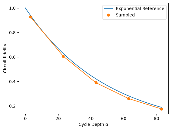
# Exponential reference
xx = np.linspace(0, fids['cycle_depth'].max())
plt.plot(xx, (1 - 5e-3) ** (4 * xx), label=r'Exponential Reference')


def _p(fids):
    plt.plot(fids['cycle_depth'], fids['fidelity'], 'o-', label=fids.name)


fids.name = 'Sampled'
_p(fids)

plt.ylabel('Circuit fidelity')
plt.xlabel('Cycle Depth $d$')
plt.legend(loc='best')
<matplotlib.legend.Legend at 0x7f652521b8d0>
Optimize PhasedFSimGate parameters
We know what circuits we requested, and in this simulated example, we know what coherent error has happened. But in a real experiment, there is likely unknown coherent error that you would like to characterize. Therefore, we make the five angles in PhasedFSimGate free parameters and use a classical optimizer to find which set of parameters best describes the data we collected from the noisy simulator (or device, if this was a real experiment).
import multiprocessing

pool = multiprocessing.get_context('spawn').Pool()
from cirq.experiments.xeb_fitting import (
    parameterize_circuit,
    characterize_phased_fsim_parameters_with_xeb,
    SqrtISwapXEBOptions,
)

# Set which angles we want to characterize (all)
options = SqrtISwapXEBOptions(
    characterize_theta=True,
    characterize_zeta=True,
    characterize_chi=True,
    characterize_gamma=True,
    characterize_phi=True,
)
# Parameterize the sqrt(iSWAP)s in our circuit library
pcircuits = [parameterize_circuit(circuit, options) for circuit in circuits]

# Run the characterization loop
characterization_result = characterize_phased_fsim_parameters_with_xeb(
    sampled_df,
    pcircuits,
    cycle_depths,
    options,
    pool=pool,
    # ease tolerance so it converges faster:
    fatol=5e-3,
    xatol=5e-3,
)
Simulating with theta =  -0.785 zeta  =       0 chi   =       0 gamma =       0 phi   =       0
Loss:   0.527
Simulating with theta =  -0.685 zeta  =       0 chi   =       0 gamma =       0 phi   =       0
Loss:   0.596
Simulating with theta =  -0.785 zeta  =     0.1 chi   =       0 gamma =       0 phi   =       0
Loss:   0.562
Simulating with theta =  -0.785 zeta  =       0 chi   =     0.1 gamma =       0 phi   =       0
Loss:   0.557
Simulating with theta =  -0.785 zeta  =       0 chi   =       0 gamma =     0.1 phi   =       0
Loss:   0.589
Simulating with theta =  -0.785 zeta  =       0 chi   =       0 gamma =       0 phi   =     0.1
Loss:   0.547
Simulating with theta =  -0.885 zeta  =    0.04 chi   =    0.04 gamma =    0.04 phi   =    0.04
Loss:   0.618
Simulating with theta =  -0.735 zeta  =    0.01 chi   =    0.01 gamma =    0.01 phi   =    0.01
Loss:   0.546
Simulating with theta =  -0.765 zeta  =   0.044 chi   =   0.044 gamma =  -0.096 phi   =   0.044
Loss:   0.582
Simulating with theta =   -0.77 zeta  =   0.033 chi   =   0.033 gamma =  -0.047 phi   =   0.033
Loss:   0.546
Simulating with theta =  -0.759 zeta  = -0.0828 chi   =  0.0572 gamma = -0.0148 phi   =  0.0572
Loss:   0.555
Simulating with theta =  -0.749 zeta  = -0.0159 chi   = -0.0599 gamma = -0.0207 phi   =  0.0801
Loss:   0.571
Simulating with theta =  -0.776 zeta  = -0.00398 chi   =    0.06 gamma = -0.00518 phi   =    0.02
Loss:   0.528
Simulating with theta =  -0.782 zeta  =  0.0984 chi   =  -0.016 gamma = -0.00207 phi   = 0.00801
Loss:   0.559
Simulating with theta =  -0.765 zeta  = -0.0375 chi   =  0.0389 gamma = -0.0116 phi   =  0.0449
Loss:   0.525
Simulating with theta =  -0.748 zeta  = 0.000609 chi   =  0.0568 gamma = -0.0215 phi   = -0.0568
Loss:   0.571
Simulating with theta =  -0.776 zeta  = 0.000152 chi   =  0.0142 gamma = -0.00538 phi   =  0.0608
Loss:   0.527
Simulating with theta =  -0.814 zeta  = -0.0133 chi   =  0.0484 gamma = -0.0377 phi   =  0.0535
Loss:    0.54
Simulating with theta =  -0.796 zeta  = -0.0549 chi   =  0.0316 gamma =  0.0231 phi   =  0.0387
Loss:   0.536
Simulating with theta =  -0.746 zeta  = -0.0251 chi   = 0.00945 gamma =   0.038 phi   =  0.0123
Loss:   0.539
Simulating with theta =  -0.763 zeta  = -0.0222 chi   =  0.0192 gamma =  0.0191 phi   =  0.0226
Loss:   0.527
Simulating with theta =   -0.75 zeta  =  0.0295 chi   =  0.0213 gamma = -0.0243 phi   =  0.0206
Loss:   0.543
Simulating with theta =  -0.785 zeta  = -0.0338 chi   =   0.029 gamma =  0.0112 phi   =  0.0342
Loss:   0.523
Simulating with theta =  -0.773 zeta  = -0.0333 chi   = -0.0195 gamma =  0.0105 phi   =   0.045
Loss:   0.541
Simulating with theta =  -0.776 zeta  = -0.0113 chi   =  0.0401 gamma = -0.00126 phi   =  0.0263
Loss:   0.521
Simulating with theta =   -0.76 zeta  = -0.0419 chi   =  0.0566 gamma = 0.00483 phi   =  0.0755
Loss:   0.541
Simulating with theta =  -0.779 zeta  = -0.0105 chi   =  0.0141 gamma = 0.00121 phi   =  0.0189
Loss:   0.523
Simulating with theta =  -0.771 zeta  = -0.0463 chi   =  0.0424 gamma =  0.0128 phi   = -0.00208
Loss:   0.526
Simulating with theta =  -0.787 zeta  = -0.0335 chi   =  0.0466 gamma = -0.0141 phi   =  0.0263
Loss:   0.525
Simulating with theta =  -0.786 zeta  = -0.00439 chi   =  0.0252 gamma = -0.0187 phi   =  0.0623
Loss:   0.522
Simulating with theta =    -0.8 zeta  = 0.000101 chi   =  0.0232 gamma = 0.00296 phi   =  0.0222
Loss:   0.525
Simulating with theta =  -0.783 zeta  =  0.0096 chi   = 0.00602 gamma =  0.0123 phi   =  0.0392
Loss:   0.529
Simulating with theta =  -0.786 zeta  = -0.0228 chi   =  0.0365 gamma = -0.00753 phi   =  0.0295
Loss:   0.521
Simulating with theta =  -0.765 zeta  = -0.0332 chi   =  0.0348 gamma = -0.00897 phi   =  0.0462
Loss:   0.525
Simulating with theta =  -0.791 zeta  = -0.00822 chi   =  0.0261 gamma = -2.36e-05 phi   =  0.0282
Loss:   0.521
Simulating with theta =  -0.782 zeta  =  0.0109 chi   =  0.0278 gamma = -0.0217 phi   =  0.0319
Loss:   0.528
Simulating with theta =  -0.784 zeta  = -0.0226 chi   =  0.0287 gamma = 0.00298 phi   =  0.0336
Loss:    0.52
Simulating with theta =   -0.79 zeta  = -0.0173 chi   =  0.0485 gamma =  -0.011 phi   =  0.0531
Loss:   0.521
Simulating with theta =  -0.785 zeta  = -0.0285 chi   =  0.0468 gamma =  0.0119 phi   = 0.00599
Loss:   0.522
Simulating with theta =  -0.786 zeta  = -0.0104 chi   =  0.0306 gamma =  -0.011 phi   =  0.0482
Loss:    0.52
Simulating with theta =  -0.777 zeta  = -0.0255 chi   =  0.0477 gamma = -0.0111 phi   =   0.048
Loss:    0.52
Simulating with theta =  -0.771 zeta  = -0.0342 chi   =  0.0585 gamma = -0.0166 phi   =  0.0579
Loss:   0.525
Simulating with theta =  -0.774 zeta  = -0.0198 chi   =   0.025 gamma = -0.000165 phi   =  0.0212
Loss:   0.522
Simulating with theta =  -0.786 zeta  = -0.0179 chi   =  0.0426 gamma = -0.0083 phi   =  0.0451
Loss:    0.52
Simulating with theta =  -0.777 zeta  = -0.0123 chi   =  0.0394 gamma = -0.00395 phi   =   0.051
Loss:   0.521
Simulating with theta =  -0.789 zeta  = -0.0242 chi   =  0.0355 gamma = -0.0113 phi   =  0.0641
Loss:   0.521
Simulating with theta =  -0.785 zeta  =  -0.021 chi   =  0.0366 gamma = -0.00879 phi   =  0.0546
Loss:    0.52
Simulating with theta =   -0.79 zeta  = -0.0266 chi   =  0.0351 gamma = -0.0105 phi   =  0.0409
Loss:   0.521
Simulating with theta =   -0.78 zeta  = -0.0159 chi   =  0.0383 gamma = -0.0056 phi   =  0.0484
Loss:    0.52
Simulating with theta =   -0.78 zeta  = -0.0307 chi   =   0.047 gamma = -0.0013 phi   =  0.0437
Loss:    0.52
Simulating with theta =  -0.779 zeta  = -0.0218 chi   =  0.0562 gamma =  -0.017 phi   =  0.0624
Loss:   0.522
Simulating with theta =  -0.783 zeta  = -0.0224 chi   =  0.0356 gamma = -0.00202 phi   =  0.0408
Loss:   0.519
Simulating with theta =  -0.788 zeta  = -0.0176 chi   =  0.0324 gamma = 0.000705 phi   =   0.045
Loss:    0.52
Simulating with theta =   -0.78 zeta  = -0.0235 chi   =  0.0439 gamma = -0.00815 phi   =  0.0473
Loss:   0.519
Simulating with theta =  -0.786 zeta  = -0.00954 chi   =  0.0318 gamma = -0.0118 phi   =  0.0508
Loss:    0.52
Simulating with theta =  -0.781 zeta  = -0.0254 chi   =  0.0432 gamma = -0.00394 phi   =  0.0455
Loss:   0.519
Simulating with theta =  -0.778 zeta  = -0.0254 chi   =  0.0364 gamma = -0.0031 phi   =  0.0496
Loss:    0.52
Simulating with theta =  -0.784 zeta  = -0.0198 chi   =  0.0411 gamma =  -0.007 phi   =  0.0462
Loss:   0.519
Simulating with theta =  -0.778 zeta  = -0.0219 chi   =  0.0442 gamma = -0.00189 phi   =  0.0366
Loss:    0.52
Simulating with theta =  -0.782 zeta  = -0.0293 chi   =  0.0448 gamma = -0.0036 phi   =  0.0381
Loss:    0.52
Simulating with theta =  -0.781 zeta  = -0.0193 chi   =    0.04 gamma = -0.0051 phi   =  0.0459
Loss:   0.519
Simulating with theta =  -0.785 zeta  = -0.0223 chi   =  0.0373 gamma = -0.00859 phi   =  0.0536
Loss:    0.52
Simulating with theta =   -0.78 zeta  =  -0.022 chi   =  0.0425 gamma = -0.00357 phi   =  0.0409
Loss:   0.519
Simulating with theta =  -0.783 zeta  =   -0.02 chi   =  0.0371 gamma = -0.000494 phi   =  0.0404
Loss:   0.519
Simulating with theta =  -0.781 zeta  = -0.0202 chi   =  0.0459 gamma = -0.00602 phi   =  0.0467
Loss:    0.52
Simulating with theta =  -0.782 zeta  = -0.0218 chi   =  0.0382 gamma = -0.00302 phi   =  0.0423
Loss:   0.519
Simulating with theta =  -0.783 zeta  = -0.0157 chi   =  0.0363 gamma = -0.00373 phi   =  0.0408
Loss:   0.519
Simulating with theta =  -0.782 zeta  =  -0.023 chi   =  0.0415 gamma = -0.00389 phi   =  0.0443
Loss:   0.519
characterization_result.final_params
{(cirq.GridQubit(4, 4),
  cirq.GridQubit(4, 5)): {'theta': np.float64(-0.7824010738176892), 'zeta': np.float64(-0.021846951021398952), 'chi': np.float64(0.03817187711394892), 'gamma': np.float64(-0.0030186313800510695), 'phi': np.float64(0.04228060788532288)} }
characterization_result.fidelities_df
from cirq.experiments.xeb_fitting import before_and_after_characterization

before_after_df = before_and_after_characterization(fids, characterization_result)
before_after_df
from cirq.experiments.xeb_fitting import exponential_decay

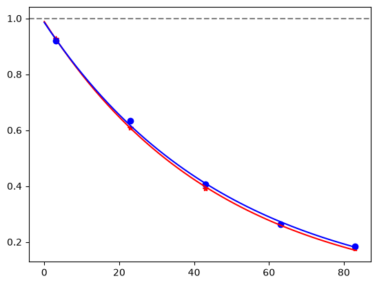
for i, row in before_after_df.iterrows():
    plt.axhline(1, color='grey', ls='--')
    plt.plot(row['cycle_depths_0'], row['fidelities_0'], '*', color='red')
    plt.plot(row['cycle_depths_c'], row['fidelities_c'], 'o', color='blue')

    xx = np.linspace(0, np.max(row['cycle_depths_0']))
    plt.plot(xx, exponential_decay(xx, a=row['a_0'], layer_fid=row['layer_fid_0']), color='red')
    plt.plot(xx, exponential_decay(xx, a=row['a_c'], layer_fid=row['layer_fid_c']), color='blue')

    plt.show()