Feature Testbed Benchmark Library

{ }

The Feature Testbed and Benchmarking Library (FTb/BL) consists of a series of workflow tools in cirq_google.workflow and a library of application-inspired algorithms conforming to those specifications living in ReCirq.

Computer code can serve as the intermediary language between algorithms researchers, software developers, and providers of quantum hardware -- each of whom have their own unique domain expertise. Higher-order abstraction in Quantum Executables can support higher-order functionality in our Quantum Runtime.

By architecting features, tools, and techniques to be part of a well specified runtime we can:

• Easily run experiments ("A/B testing") on the impact of features by toggling them in the runtime and running against a full library of applications.
• Create a clear specification for how to leverage a feature, tool, or technique in our library of applications.
• Mock out runtime features for ease of testing without consuming the scarce resource of quantum computer time.

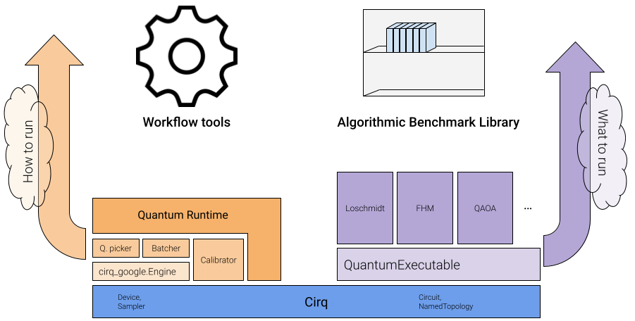
Algorithmic Benchmark Library

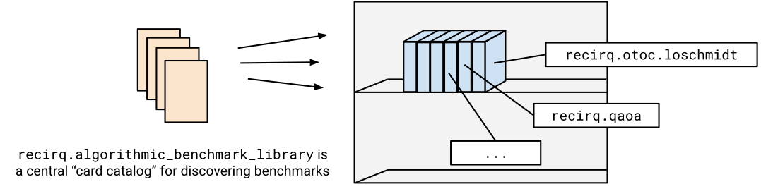
The algorithmic benchmark library is a collection of quantum executables that probe different aspects of a quantum computer's performance. Each benchmark is based off of an algorithm of interest and operates on > 2 qubits (in contrast to traditional 1- and 2-qubit fidelity metrics).

We use the library card catalog in recirq.algorithmic_benchmark_library to get a description of each algorithmic benchmark.

try:
    import recirq
except ImportError:
    !pip install --quiet git+https://github.com/quantumlib/ReCirq

import recirq.algorithmic_benchmark_library as algos
from IPython.display import display

for algo in algos.BENCHMARKS:
    display(algo)

Select an example benchmark using executable_family

Each benchmark has a name (e.g. "loschmidt.tilted_square_lattice") and a domain (e.g. this benchmark is inspired by the OTOC Experiment so it is given the domain of "recirq.otoc"). We combine these two properties to give the executable_family string, which serves as a globally-unique identifier for each benchmark. In ReCirq, the executable_family is the Python module path where the relevant code can be found.

We'll seelct the "recirq.otoc.loschmidt.tilted_square_lattice" benchmark by querying the card catalog using this unique executable_family identifier.

algo = algos.get_algo_benchmark_by_executable_family(
    executable_family='recirq.otoc.loschmidt.tilted_square_lattice')
print(type(algo))
algo

<class 'recirq.algorithmic_benchmark_library.AlgorithmicBenchmark'>

from pathlib import Path

# In ReCirq, the `executable_family` is the Python module path where
# the relevant code can be found.
algo_src_dir = Path('..') / algo.executable_family.replace('.', '/')
algo_src_dir

PosixPath('../recirq/otoc/loschmidt/tilted_square_lattice')

Each AlgorithmicBenchmark has a collection of BenchmarkConfigs

An algorithmic benchmark defines a class of quantum executables. Often times the specific size, shape, depth or other properties is left as a parameter. For each benchmark, we have a collection of BenchmarkConfigs that fully specify what to run and can be run repeatedly for controlled comparison over time or between processors.

for config in algo.configs:
    print(config.full_name)

loschmidt.tilted_square_lattice.small-v1
loschmidt.tilted_square_lattice.small-cz-v1

We'll select the small-cz-v1 configuration, as described below.

config = algo.get_config_by_full_name('loschmidt.tilted_square_lattice.small-cz-v1')
print(config.description)

A 'small' configuration for quick verification of Loschmidt echos using the 
CZ gate

This configuration uses small grid topologies (making it suitable for
running on simulators) and a small number of random instances making it
suitable for getting a quick reading on processor performance in ~minutes.

A benchmark has three steps:

1. Executable generation
2. Execution
3. Analysis

Usually, these steps are done in order but independently and with differing frequencies. For a robust benchmark, executable generation should likely be done once and the serialized QuantumExecutableGroup cached and re-used for subsequent executions. Execution should happen on a regular cadence for historical data or as part of an A/B test for trialing different runtime configuraiton options. Analysis can happen at any moment and may incorperate the latest data or a collection of datasets across time, processors, or runtime configurations.

config

BenchmarkConfig(short_name='small-cz-v1', full_name='loschmidt.tilted_square_lattice.small-cz-v1', gen_script='gen-small-cz-v1.py', run_scripts=['run-simulator-cz.py'], description="A 'small' configuration for quick verification of Loschmidt echos using the \nCZ gate\n\nThis configuration uses small grid topologies (making it suitable for\nrunning on simulators) and a small number of random instances making it\nsuitable for getting a quick reading on processor performance in ~minutes.")

Step 1: Executable Generation

Here, we generate a QuantumExecutableGroup for a given range of parameters. This step is usually done once for each BenchmarkConfig and the serialized result is saved and re-used for execution. We use a short python file more like a configuration file than a script to commit the parameters for a particular config. The filename can be found as config.gen_script.

# Helper function to show scripts from the ReCirq repository for comparison
from IPython.display import Code, HTML

def show_python_script(path: Path):
    with path.open() as f:
        contents = f.read()

    display(HTML(f"<u>The contents of {path}:</u>"))
    display(Code(contents[contents.find('import'):], language='python'))

show_python_script(algo_src_dir / config.gen_script)

We've copied the important bit into the cell below so you can execute it within this notebook.

import numpy as np
from recirq.otoc.loschmidt.tilted_square_lattice import get_all_tilted_square_lattice_executables

exes = get_all_tilted_square_lattice_executables(
    min_side_length=2, max_side_length=3, side_length_step=1,
    n_instances=3,
    macrocycle_depths=np.arange(0, 4 + 1, 1),
    twoq_gate_name='cz',
    seed=52,
)
len(exes)

45

Step 2: Execution

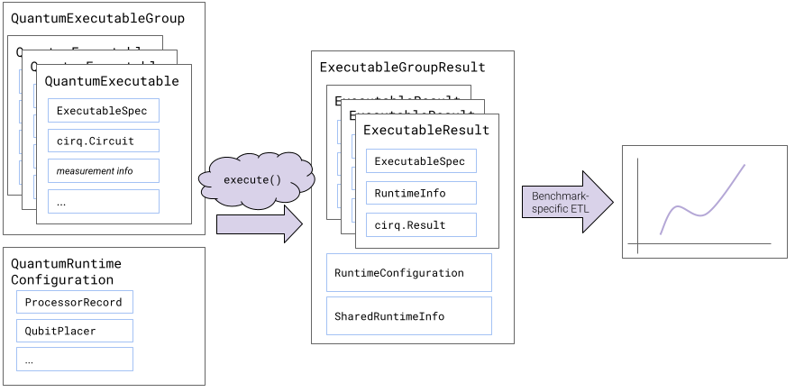
The QuantumExecutableGroup for our benchmark defines what to run. Now we configure how to run it. This is done with a QuantumRuntimeConfiguration.

We specify which processor to use (here: a simulated one. Try changing to EngineProcessorRecord to run on a real device), how to map the "logical" qubit identities in the problem to physical qubits (here: randomly), and how to set the random number generator's seed.

from cirq_google.workflow import (
    QuantumRuntimeConfiguration, 
    SimulatedProcessorWithLocalDeviceRecord,
    EngineProcessorRecord,
    RandomDevicePlacer
)

rt_config = QuantumRuntimeConfiguration(
    processor_record=SimulatedProcessorWithLocalDeviceRecord('rainbow', noise_strength=0.005),
    qubit_placer=RandomDevicePlacer(),
    random_seed=52,
)
rt_config

cirq_google.QuantumRuntimeConfiguration(processor_record=cirq_google.SimulatedProcessorWithLocalDeviceRecord(processor_id='rainbow', noise_strength=0.005), run_id=None, random_seed=52, qubit_placer=cirq_google.RandomDevicePlacer())

Again, we use a short Python file in the repository to commit the configuration options for a particular config.

show_python_script(algo_src_dir / 'run-simulator.py')

Usually, we're very careful about saving everything in a structured way relative to a base_data_dir. Since this notebook is run interactively, we'll make a temporary directory to serve as our base_data_dir.

import tempfile
base_data_dir = tempfile.mkdtemp()
base_data_dir

'/tmp/tmppw19om17'

Actual execution is as simple as calling execute once the runtime configuration and executables are created.

from cirq_google.workflow import execute
raw_results = execute(rt_config, exes, base_data_dir=base_data_dir)

45 / 45

Since we didn't input our own, a random run_id is generated for us. The run_ids must be unique within a data directory.

run_id = raw_results.shared_runtime_info.run_id
run_id

'3cb7656c-eee1-436c-8a05-0affb09863ed'

Step 3: Analysis and Plotting

Finally, we can analyze one or more datasets and generate plots. Since we've decoupled problem generation and execution from this step you can slice and dice your data any way you want. Usually, analysis routines will use the accompanying analysis module for helper function and do much of the pd.DataFrame and matplotlib munging interactively in a Jupyter notebook. One of the plots from plots.ipynb is reproduced here.

import recirq.otoc.loschmidt.tilted_square_lattice.analysis as analysis
import cirq_google as cg
import pandas as pd

raw_results = cg.ExecutableGroupResultFilesystemRecord.from_json(run_id=run_id, base_data_dir=base_data_dir)\
                    .load(base_data_dir=base_data_dir)
df = analysis.loschmidt_results_to_dataframe(raw_results)
df.head()

vs_depth_df, vs_depth_gb_cols = analysis.agg_vs_macrocycle_depth(df)
fit_df, exp_ansatz = analysis.fit_vs_macrocycle_depth(df)
total_df = pd.merge(vs_depth_df, fit_df, on=vs_depth_gb_cols)

from matplotlib import pyplot as plt

colors = plt.get_cmap('tab10')

for i, row in total_df.iterrows():
    plt.errorbar(
        x=row['macrocycle_depth'],
        y=row['success_probability_mean'],
        yerr=row['success_probability_std'],
        marker='o', capsize=5, ls='',
        color=colors(i),
        label=f'{row["width"]}x{row["height"]} ({row["n_qubits"]}q) {row["processor_str"]}; f={row["f"]:.3f}'
    )

    xx = np.linspace(np.min(row['macrocycle_depth']), np.max(row['macrocycle_depth']))
    yy = exp_ansatz(xx, a=row['a'], f=row['f'])
    plt.plot(xx, yy, ls='--', color=colors(i))

plt.legend(loc='best')
plt.yscale('log')
plt.xlabel('Macrocycle Depth')
plt.ylabel('Success Probability')
plt.tight_layout()

Appendix: QuantumExecutable and ExecutableSpec

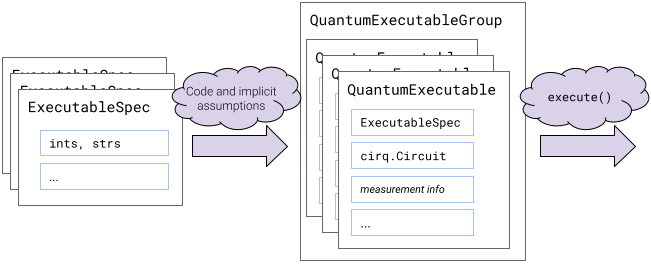
• A QuantumExecutable contains a complete description of what to run. Think of it as a souped-up version of a cirq.Circuit.
• An ExecutableSpec is a problem-specific dataclass minimally capturing the salient independent variables, usually with plain-old-datatypes suitable for databasing and plotting.

Each benchmark provides a problem-specific subclass of ExecutableSpec and a function that turns those specs into problem-agnostic, fully-specified QuantumExecutables.

QuantumExecutable

Each QuantumExecutable fully specifies the quantum program to be run, but as high-level as possible. The most familiar part is circuit: cirq.Circuit, but the executable also includes measurement (i.e. repetitions) information, sweep parameters, and other data. We'll look at the fields on one of our executables below:

# Pick one `QuantumExecutable` from the `QuantumExecutableGroup` 
exe = exes.executables[0]

import dataclasses
print('exe fields:')
print([f.name for f in dataclasses.fields(exe)])

exe fields:
['circuit', 'measurement', 'params', 'spec', 'problem_topology', 'initial_state']

QuantumExectutable.spec is a reference to the ExecutableSpec used to create this executable. Here, it is a TiltedSquareLatticeLoschmidtSpec which derives from the ExecutableSpec base class. Each AlgorithmicBenchmark has its own class derived from ExecutableSpec. This correspondance is recorded as AlgorithmicBenchmark.spec_class.

print(algo.spec_class)
print(exe.spec.__class__)

<class 'recirq.otoc.loschmidt.tilted_square_lattice.tilted_square_lattice.TiltedSquareLatticeLoschmidtSpec'>
<class 'recirq.otoc.loschmidt.tilted_square_lattice.tilted_square_lattice.TiltedSquareLatticeLoschmidtSpec'>

ExecutableSpec

The ExecutableSpec is a problem-specific dataclass containing the relevant independent variables for a benchmark. Since each benchmark has its own subclass of ExecutableSpec, we'll continue using our example loschmidt benchmark and create an example TiltedSquareLatticeLoschmidtSpec:

import cirq
from recirq.otoc.loschmidt.tilted_square_lattice import TiltedSquareLatticeLoschmidtSpec

spec = TiltedSquareLatticeLoschmidtSpec(
    topology=cirq.TiltedSquareLattice(width=2, height=2),
    macrocycle_depth=0,
    instance_i=0,
    n_repetitions=1_000,
    twoq_gate_name='cz'
)

I've chosen the parameters corresponding to our example executable, exe = exes.executables[0].

exe.spec == spec

True

Below, we re-create the executable using just the spec.

from recirq.otoc.loschmidt.tilted_square_lattice import tilted_square_lattice_spec_to_exe

exe2 = tilted_square_lattice_spec_to_exe(exe.spec, rs=np.random.RandomState(52))
exe == exe2

True