|
|
|
|
|
try:
    import cirq
except ImportError:
    print("installing cirq...")
    !pip install --quiet cirq
    print("installed cirq.")
This notebook demonstrates how to use the functionality in cirq.experiments to run Isolated XEB end-to-end. "Isolated" means we do one pair of qubits at a time.
import cirq
import numpy as np
Set up Random Circuits
We create a library of 20 random, two-qubit circuits using the sqrt(ISWAP) gate on the two qubits we've chosen.
from cirq.experiments import random_quantum_circuit_generation as rqcg

circuits = rqcg.generate_library_of_2q_circuits(
    n_library_circuits=20,
    two_qubit_gate=cirq.ISWAP**0.5,
    q0=cirq.GridQubit(4, 4),
    q1=cirq.GridQubit(4, 5),
)
print(len(circuits))
20
# We will truncate to these lengths
max_depth = 100
cycle_depths = np.arange(3, max_depth, 20)
cycle_depths
array([ 3, 23, 43, 63, 83])
Set up a Sampler.
For demonstration, we'll use a density matrix simulator to sample noisy samples. However, input a device_name (and have an authenticated Google Cloud project name set as your GOOGLE_CLOUD_PROJECT environment variable) to run on a real device.
device_name = None  # change me!

if device_name is None:
    sampler = cirq.DensityMatrixSimulator(noise=cirq.depolarize(5e-3))
else:
    import cirq_google as cg

    sampler = cg.get_engine_sampler(device_name, gate_set_name='sqrt_iswap')
    device = cg.get_engine_device(device_name)

    import cirq.contrib.routing as ccr

    graph = ccr.gridqubits_to_graph_device(device.qubits)
    pos = {q: (q.row, q.col) for q in graph.nodes}
    import networkx as nx

    nx.draw_networkx(graph, pos=pos)
Take Data
from cirq.experiments.xeb_sampling import sample_2q_xeb_circuits

sampled_df = sample_2q_xeb_circuits(
    sampler=sampler, circuits=circuits, cycle_depths=cycle_depths, repetitions=10_000
)
sampled_df
100%|██████████| 108/108 [00:18<00:00, 5.93it/s]
Benchmark fidelities
from cirq.experiments.xeb_fitting import benchmark_2q_xeb_fidelities

fids = benchmark_2q_xeb_fidelities(
    sampled_df=sampled_df, circuits=circuits, cycle_depths=cycle_depths
)
fids
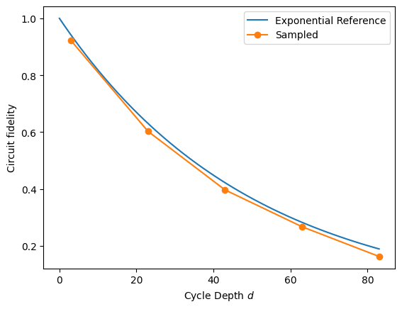
%matplotlib inline
from matplotlib import pyplot as plt

# Exponential reference
xx = np.linspace(0, fids['cycle_depth'].max())
plt.plot(xx, (1 - 5e-3) ** (4 * xx), label=r'Exponential Reference')


def _p(fids):
    plt.plot(fids['cycle_depth'], fids['fidelity'], 'o-', label=fids.name)


fids.name = 'Sampled'
_p(fids)

plt.ylabel('Circuit fidelity')
plt.xlabel('Cycle Depth $d$')
plt.legend(loc='best')
<matplotlib.legend.Legend at 0x7f4a4e57d2a0>
Optimize PhasedFSimGate parameters
We know what circuits we requested, and in this simulated example, we know what coherent error has happened. But in a real experiment, there is likely unknown coherent error that you would like to characterize. Therefore, we make the five angles in PhasedFSimGate free parameters and use a classical optimizer to find which set of parameters best describes the data we collected from the noisy simulator (or device, if this was a real experiment).
import multiprocessing

pool = multiprocessing.get_context('spawn').Pool()
from cirq.experiments.xeb_fitting import (
    parameterize_circuit,
    characterize_phased_fsim_parameters_with_xeb,
    SqrtISwapXEBOptions,
)

# Set which angles we want to characterize (all)
options = SqrtISwapXEBOptions(
    characterize_theta=True,
    characterize_zeta=True,
    characterize_chi=True,
    characterize_gamma=True,
    characterize_phi=True,
)
# Parameterize the sqrt(iswap)s in our circuit library
pcircuits = [parameterize_circuit(circuit, options) for circuit in circuits]

# Run the characterization loop
characterization_result = characterize_phased_fsim_parameters_with_xeb(
    sampled_df,
    pcircuits,
    cycle_depths,
    options,
    pool=pool,
    # ease tolerance so it converges faster:
    fatol=5e-3,
    xatol=5e-3,
)
Simulating with theta =  -0.785 zeta  =       0 chi   =       0 gamma =       0 phi   =       0
Loss:   0.531
Simulating with theta =  -0.685 zeta  =       0 chi   =       0 gamma =       0 phi   =       0
Loss:   0.581
Simulating with theta =  -0.785 zeta  =     0.1 chi   =       0 gamma =       0 phi   =       0
Loss:   0.564
Simulating with theta =  -0.785 zeta  =       0 chi   =     0.1 gamma =       0 phi   =       0
Loss:   0.553
Simulating with theta =  -0.785 zeta  =       0 chi   =       0 gamma =     0.1 phi   =       0
Loss:   0.595
Simulating with theta =  -0.785 zeta  =       0 chi   =       0 gamma =       0 phi   =     0.1
Loss:   0.564
Simulating with theta =  -0.745 zeta  =    0.04 chi   =    0.04 gamma =    -0.1 phi   =    0.04
Loss:    0.61
Simulating with theta =  -0.775 zeta  =    0.01 chi   =    0.01 gamma =    0.05 phi   =    0.01
Loss:   0.554
Simulating with theta =  -0.881 zeta  =   0.044 chi   =   0.044 gamma =    0.02 phi   =   0.044
Loss:   0.601
Simulating with theta =  -0.734 zeta  =   0.011 chi   =   0.011 gamma =   0.005 phi   =   0.011
Loss:   0.543
Simulating with theta =  -0.761 zeta  =  0.0484 chi   =  0.0484 gamma =   0.022 phi   = -0.0916
Loss:   0.572
Simulating with theta =  -0.779 zeta  =  0.0121 chi   =  0.0121 gamma =  0.0055 phi   =  0.0521
Loss:   0.544
Simulating with theta =  -0.759 zeta  = -0.0868 chi   =  0.0532 gamma =  0.0242 phi   =  0.0292
Loss:   0.578
Simulating with theta =  -0.779 zeta  =  0.0533 chi   =  0.0133 gamma = 0.00605 phi   = 0.00731
Loss:   0.539
Simulating with theta =   -0.77 zeta  =  0.0206 chi   =  0.0446 gamma = -0.0434 phi   =  0.0182
Loss:   0.551
Simulating with theta =  -0.754 zeta  =  0.0388 chi   = -0.0676 gamma = -0.0107 phi   =  0.0354
Loss:   0.564
Simulating with theta =  -0.777 zeta  =  0.0097 chi   =  0.0581 gamma = -0.00268 phi   = 0.00886
Loss:   0.535
Simulating with theta =  -0.772 zeta  =  0.0139 chi   = -0.00676 gamma =  0.0489 phi   =  0.0135
Loss:   0.559
Simulating with theta =   -0.77 zeta  =  0.0189 chi   =  0.0317 gamma = -0.0203 phi   =   0.017
Loss:   0.534
Simulating with theta =  -0.759 zeta  =  0.0251 chi   =  0.0336 gamma = -0.0103 phi   = -0.0344
Loss:    0.55
Simulating with theta =  -0.774 zeta  =  0.0153 chi   =  0.0175 gamma = 0.00156 phi   =  0.0305
Loss:   0.534
Simulating with theta =   -0.82 zeta  =  0.0279 chi   =  0.0372 gamma = -0.0112 phi   =  0.0145
Loss:   0.548
Simulating with theta =  -0.756 zeta  =  0.0152 chi   =  0.0176 gamma = 0.000962 phi   =  0.0119
Loss:   0.533
Simulating with theta =  -0.767 zeta  = -0.0296 chi   =  0.0366 gamma = -0.0142 phi   =    0.02
Loss:   0.536
Simulating with theta =   -0.77 zeta  = -0.00891 chi   =  0.0308 gamma = -0.00917 phi   =  0.0168
Loss:   0.531
Simulating with theta =  -0.765 zeta  = 0.00652 chi   = -0.0191 gamma = -0.0081 phi   =  0.0216
Loss:   0.537
Simulating with theta =  -0.774 zeta  =  0.0089 chi   =  0.0388 gamma = -0.00404 phi   =   0.012
Loss:   0.531
Simulating with theta =  -0.773 zeta  = -0.00667 chi   =  0.0101 gamma =   0.016 phi   =  0.0115
Loss:   0.533
Simulating with theta =  -0.769 zeta  = -0.0119 chi   =  0.0215 gamma = -4.04e-05 phi   = -0.0096
Loss:   0.529
Simulating with theta =  -0.767 zeta  = -0.0256 chi   =  0.0234 gamma = -0.000839 phi   = -0.0296
Loss:   0.533
Simulating with theta =  -0.768 zeta  = 0.00799 chi   =  0.0333 gamma = -0.0209 phi   = 0.000983
Loss:   0.536
Simulating with theta =  -0.772 zeta  =  -0.003 chi   =  0.0159 gamma = 0.00679 phi   = 0.00884
Loss:    0.53
Simulating with theta =  -0.792 zeta  = -0.0212 chi   =  0.0252 gamma = -0.00354 phi   = -0.000627
Loss:   0.533
Simulating with theta =  -0.765 zeta  = 0.00612 chi   =  0.0195 gamma = -0.000165 phi   = 0.00874
Loss:    0.53
Simulating with theta =  -0.777 zeta  = 0.00895 chi   = 0.00746 gamma =  0.0102 phi   = -0.00879
Loss:   0.529
Simulating with theta =   -0.78 zeta  =  0.0179 chi   = -0.00421 gamma =  0.0199 phi   = -0.0216
Loss:   0.531
Simulating with theta =  -0.757 zeta  = 0.00362 chi   =  0.0412 gamma = 0.00509 phi   =  0.0045
Loss:   0.532
Simulating with theta =  -0.778 zeta  = 0.000905 chi   =  0.0103 gamma = 0.00127 phi   = 0.00112
Loss:   0.529
Simulating with theta =   -0.77 zeta  = -0.00848 chi   = -0.00896 gamma =  0.0113 phi   = -0.0119
Loss:   0.533
Simulating with theta =  -0.773 zeta  = 0.00456 chi   =  0.0269 gamma = -0.000214 phi   = 0.00605
Loss:   0.529
Simulating with theta =  -0.773 zeta  = 0.00645 chi   =  0.0183 gamma = -0.00237 phi   = -0.00983
Loss:   0.529
Simulating with theta =  -0.783 zeta  = -0.00254 chi   =  0.0143 gamma =  0.0037 phi   = -0.0172
Loss:   0.528
Simulating with theta =  -0.792 zeta  = -0.00688 chi   =  0.0117 gamma = 0.00563 phi   = -0.0301
Loss:    0.53
Simulating with theta =  -0.785 zeta  =  0.0192 chi   = 0.00944 gamma = 0.00507 phi   = -0.00184
Loss:    0.53
Simulating with theta =  -0.773 zeta  = -0.00413 chi   =  0.0184 gamma = 0.00124 phi   = -0.00766
Loss:   0.528
Simulating with theta =  -0.773 zeta  = 0.00441 chi   =  0.0238 gamma = 0.00374 phi   = -0.0161
Loss:   0.528
Simulating with theta =  -0.771 zeta  = 0.00616 chi   =  0.0306 gamma = 0.00497 phi   = -0.0247
Loss:   0.529
Simulating with theta =  -0.779 zeta  = -0.00195 chi   =   0.018 gamma = 0.00983 phi   = -0.00762
Loss:   0.528
Simulating with theta =  -0.782 zeta  = -0.00615 chi   =  0.0179 gamma =  0.0159 phi   = -0.00652
Loss:   0.529
Simulating with theta =  -0.781 zeta  = -0.00266 chi   = 0.00596 gamma =  0.0117 phi   =  -0.029
Loss:   0.528
Simulating with theta =  -0.779 zeta  = -0.0117 chi   =  0.0248 gamma = 0.00189 phi   = -0.0222
Loss:   0.529
Simulating with theta =  -0.778 zeta  = -0.00654 chi   =  0.0204 gamma = 0.00396 phi   = -0.0189
Loss:   0.528
Simulating with theta =  -0.785 zeta  = 0.000411 chi   =  0.0146 gamma =  0.0119 phi   = -0.0278
Loss:   0.527
Simulating with theta =  -0.791 zeta  = 0.00268 chi   =  0.0126 gamma =  0.0173 phi   = -0.0379
Loss:   0.528
Simulating with theta =  -0.779 zeta  = 0.000178 chi   =  0.0305 gamma = 0.00158 phi   = -0.00603
Loss:   0.528
Simulating with theta =  -0.774 zeta  = 0.00115 chi   =  0.0287 gamma = 0.00872 phi   = -0.0134
Loss:   0.527
Simulating with theta =  -0.777 zeta  = -0.00119 chi   =  0.0117 gamma =  0.0137 phi   = -0.0275
Loss:   0.528
Simulating with theta =  -0.784 zeta  = -0.00766 chi   =  0.0136 gamma =  0.0155 phi   =  -0.022
Loss:   0.528
Simulating with theta =  -0.781 zeta  = 0.00284 chi   =  0.0142 gamma =  0.0199 phi   = -0.0205
Loss:   0.527
Simulating with theta =  -0.782 zeta  = 0.000175 chi   =   0.015 gamma =  0.0181 phi   = -0.0368
Loss:   0.527
Simulating with theta =  -0.783 zeta  = 0.00124 chi   =  0.0135 gamma =  0.0222 phi   = -0.0515
Loss:   0.528
Simulating with theta =  -0.776 zeta  = 0.00901 chi   =  0.0201 gamma =  0.0134 phi   = -0.0284
Loss:   0.527
Simulating with theta =  -0.782 zeta  = 0.00662 chi   =  0.0253 gamma =  0.0151 phi   = -0.0233
Loss:   0.527
Simulating with theta =  -0.784 zeta  =  0.0105 chi   =  0.0321 gamma =  0.0158 phi   = -0.0212
Loss:   0.527
Simulating with theta =  -0.786 zeta  = -0.00453 chi   =   0.019 gamma =  0.0161 phi   = -0.0203
Loss:   0.527
Simulating with theta =  -0.782 zeta  = -0.00131 chi   =  0.0269 gamma = 0.00807 phi   = -0.0282
Loss:   0.528
Simulating with theta =  -0.782 zeta  =  0.0018 chi   =  0.0174 gamma =   0.017 phi   = -0.0224
Loss:   0.527
Simulating with theta =  -0.792 zeta  = 0.000646 chi   = 0.00784 gamma =  0.0226 phi   = -0.0389
Loss:   0.528
Simulating with theta =  -0.779 zeta  = 0.00102 chi   =  0.0235 gamma =  0.0122 phi   = -0.0198
Loss:   0.527
Simulating with theta =  -0.779 zeta  = 0.00163 chi   =  0.0255 gamma =  0.0194 phi   = -0.0212
Loss:   0.527
Simulating with theta =  -0.777 zeta  = 0.00223 chi   =   0.031 gamma =  0.0232 phi   =  -0.018
Loss:   0.527
Simulating with theta =  -0.775 zeta  = 0.00903 chi   =  0.0237 gamma =  0.0166 phi   = -0.0291
Loss:   0.527
Simulating with theta =  -0.778 zeta  = 0.00564 chi   =  0.0225 gamma =  0.0165 phi   = -0.0269
Loss:   0.527
Simulating with theta =  -0.778 zeta  = 0.00651 chi   =  0.0306 gamma =   0.014 phi   = -0.00861
Loss:   0.528
Simulating with theta =  -0.781 zeta  = 0.00176 chi   =  0.0189 gamma =  0.0171 phi   = -0.0298
Loss:   0.527
Simulating with theta =  -0.778 zeta  = 0.00486 chi   =  0.0289 gamma =  0.0152 phi   =  -0.026
Loss:   0.527
Simulating with theta =   -0.78 zeta  = 0.00718 chi   =   0.025 gamma =  0.0211 phi   = -0.0311
Loss:   0.526
Simulating with theta =  -0.781 zeta  =  0.0103 chi   =  0.0258 gamma =  0.0256 phi   = -0.0368
Loss:   0.527
Simulating with theta =  -0.777 zeta  = 0.00181 chi   =   0.023 gamma =  0.0206 phi   = -0.0307
Loss:   0.526
Simulating with theta =  -0.774 zeta  = -0.000604 chi   =  0.0219 gamma =  0.0233 phi   = -0.0344
Loss:   0.527
Simulating with theta =   -0.78 zeta  = 0.00234 chi   =  0.0171 gamma =  0.0227 phi   = -0.0299
Loss:   0.527
Simulating with theta =  -0.781 zeta  = 0.000245 chi   =  0.0213 gamma =  0.0239 phi   = -0.0302
Loss:   0.526
Simulating with theta =  -0.783 zeta  = -0.00245 chi   =  0.0207 gamma =  0.0276 phi   = -0.0318
Loss:   0.526
Simulating with theta =   -0.78 zeta  = 0.00371 chi   =  0.0166 gamma =  0.0227 phi   = -0.0395
Loss:   0.527
Simulating with theta =   -0.78 zeta  = 0.00215 chi   =  0.0233 gamma =  0.0203 phi   = -0.0258
Loss:   0.526
Simulating with theta =  -0.779 zeta  = 0.00291 chi   =  0.0276 gamma =  0.0185 phi   = -0.0291
Loss:   0.526
Simulating with theta =  -0.778 zeta  = 0.00396 chi   =  0.0292 gamma =  0.0247 phi   =  -0.029
Loss:   0.526
Simulating with theta =  -0.779 zeta  = 0.00341 chi   =  0.0266 gamma =  0.0228 phi   = -0.0292
Loss:   0.526
Simulating with theta =  -0.778 zeta  = -0.00298 chi   =  0.0237 gamma =  0.0212 phi   = -0.0269
Loss:   0.526
Simulating with theta =  -0.778 zeta  = -0.000436 chi   =   0.024 gamma =  0.0212 phi   =  -0.028
Loss:   0.526
characterization_result.final_params
{(cirq.GridQubit(4, 4),
  cirq.GridQubit(4, 5)): {'theta': np.float64(-0.7783379736657015), 'zeta': np.float64(-0.00043573822845567947), 'chi': np.float64(0.0240391542895369), 'gamma': np.float64(0.021218997340166138), 'phi': np.float64(-0.027952516833367733)} }
characterization_result.fidelities_df
from cirq.experiments.xeb_fitting import before_and_after_characterization

before_after_df = before_and_after_characterization(fids, characterization_result)
before_after_df
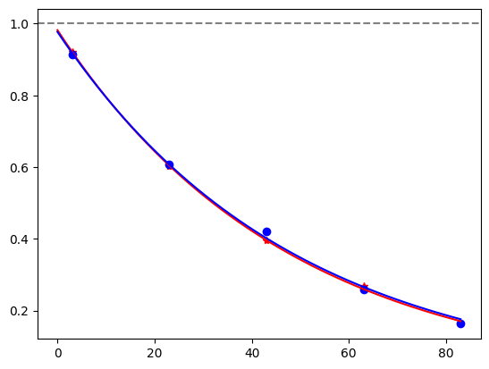
from cirq.experiments.xeb_fitting import exponential_decay

for i, row in before_after_df.iterrows():
    plt.axhline(1, color='grey', ls='--')
    plt.plot(row['cycle_depths_0'], row['fidelities_0'], '*', color='red')
    plt.plot(row['cycle_depths_c'], row['fidelities_c'], 'o', color='blue')

    xx = np.linspace(0, np.max(row['cycle_depths_0']))
    plt.plot(xx, exponential_decay(xx, a=row['a_0'], layer_fid=row['layer_fid_0']), color='red')
    plt.plot(xx, exponential_decay(xx, a=row['a_c'], layer_fid=row['layer_fid_c']), color='blue')

    plt.show()