 View on QuantumAI View on QuantumAI
|
 Run in Google Colab Run in Google Colab
|
 View source on GitHub View source on GitHub
|
|
try:
    import cirq
except ImportError:
    print("installing cirq...")
    !pip install --quiet cirq
    import cirq

    print("installed cirq.")
Cross-Entropy Benchmarking (XEB) uses the properties of random quantum programs to determine the fidelity of a wide variety of circuits. When applied to circuits with many qubits, XEB can characterize the performance of a large device. When applied to deep, two-qubit circuits it can be used to accurately characterize a two-qubit interaction potentially leading to better calibration.
# Standard imports
import numpy as np

from cirq.contrib.svg import SVGCircuit
The action of random circuits with noise
An XEB experiment collects data from the execution of random circuits subject to noise. The effect of applying a random circuit with unitary \(U\) is modeled as \(U\) followed by a depolarizing channel. The result is that the initial state \(|𝜓⟩\) is mapped to a density matrix \(ρ_U\) as follows:
\[ |𝜓⟩ → ρ_U = f |𝜓_U⟩⟨𝜓_U| + (1 - f) I / D \]
where \(|𝜓_U⟩ = U|𝜓⟩\), \(D\) is the dimension of the Hilbert space, \(I / D\) is the maximally mixed state, and \(f\) is the fidelity with which the circuit is applied.
For this model to be accurate, we require \(U\) to be a random circuit that scrambles errors. In practice, we use a particular circuit ansatz consisting of random single-qubit rotations interleaved with entangling gates.
Possible single-qubit rotations
Geometrically, we choose 8 axes in the XY plane to perform a quarter-turn (pi/2 rotation) around. This is followed by a rotation around the Z axis of 8 different magnitudes.
These 8*8 possible rotations are chosen randomly when constructing the circuit.
exponents = np.linspace(0, 7 / 4, 8)
exponents
array([0. , 0.25, 0.5 , 0.75, 1. , 1.25, 1.5 , 1.75])
import itertools

SINGLE_QUBIT_GATES = [
    cirq.PhasedXZGate(x_exponent=0.5, z_exponent=z, axis_phase_exponent=a)
    for a, z in itertools.product(exponents, repeat=2)
]
SINGLE_QUBIT_GATES[:10], '...'
([cirq.PhasedXZGate(axis_phase_exponent=0.0, x_exponent=0.5, z_exponent=0.0),
  cirq.PhasedXZGate(axis_phase_exponent=0.0, x_exponent=0.5, z_exponent=0.25),
  cirq.PhasedXZGate(axis_phase_exponent=0.0, x_exponent=0.5, z_exponent=0.5),
  cirq.PhasedXZGate(axis_phase_exponent=0.0, x_exponent=0.5, z_exponent=0.75),
  cirq.PhasedXZGate(axis_phase_exponent=0.0, x_exponent=0.5, z_exponent=1.0),
  cirq.PhasedXZGate(axis_phase_exponent=0.0, x_exponent=0.5, z_exponent=1.25),
  cirq.PhasedXZGate(axis_phase_exponent=0.0, x_exponent=0.5, z_exponent=1.5),
  cirq.PhasedXZGate(axis_phase_exponent=0.0, x_exponent=0.5, z_exponent=1.75),
  cirq.PhasedXZGate(axis_phase_exponent=0.25, x_exponent=0.5, z_exponent=0.0),
  cirq.PhasedXZGate(axis_phase_exponent=0.25, x_exponent=0.5, z_exponent=0.25)],
 '...')
Random circuit
We use cirq.experiments.random_quantum_circuit_generation.random_rotations_between_two_qubit_circuit to generate a random two-qubit circuit. Note that we provide the possible single-qubit rotations from above and declare that our two-qubit operation is the \(\sqrt{i\mathrm{SWAP} }\) gate.
import cirq_google as cg
from cirq.experiments import random_quantum_circuit_generation as rqcg

q0, q1 = cirq.LineQubit.range(2)
circuit = rqcg.random_rotations_between_two_qubit_circuit(
    q0,
    q1,
    depth=4,
    two_qubit_op_factory=lambda a, b, _: cirq.SQRT_ISWAP(a, b),
    single_qubit_gates=SINGLE_QUBIT_GATES,
)
SVGCircuit(circuit)
Estimating fidelity
Let \(O_U\) be an observable that is diagonal in the computational basis. Then the expectation value of \(O_U\) on \(ρ_U\) is given by
\[ Tr(ρ_U O_U) = f ⟨𝜓_U|O_U|𝜓_U⟩ + (1 - f) Tr(O_U / D). \]
This equation shows how \(f\) can be estimated, since \(Tr(ρ_U O_U)\) can be estimated from experimental data, and \(⟨𝜓_U|O_U|𝜓_U⟩\) and \(Tr(O_U / D)\) can be computed.
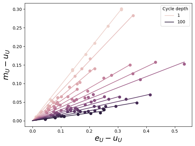
Let \(e_U = ⟨𝜓_U|O_U|𝜓_U⟩\), \(u_U = Tr(O_U / D)\), and \(m_U\) denote the experimental estimate of \(Tr(ρ_U O_U)\). We can write the following linear equation (equivalent to the expression above):
\[ m_U = f e_U + (1-f) u_U \\ m_U - u_U = f (e_U - u_U) \]
# Make long circuits (which we will truncate)
MAX_DEPTH = 100
N_CIRCUITS = 10
circuits = [
    rqcg.random_rotations_between_two_qubit_circuit(
        q0,
        q1,
        depth=MAX_DEPTH,
        two_qubit_op_factory=lambda a, b, _: cirq.SQRT_ISWAP(a, b),
        single_qubit_gates=SINGLE_QUBIT_GATES,
    )
    for _ in range(N_CIRCUITS)
]
# We will truncate to these lengths
cycle_depths = np.arange(1, MAX_DEPTH + 1, 9)
cycle_depths
array([ 1, 10, 19, 28, 37, 46, 55, 64, 73, 82, 91, 100])
Execute circuits
Cross-Entropy Benchmarking (XEB) requires sampled bitstrings from the device being benchmarked as well as the true probabilities from a noiseless simulation. We find these quantities for all (cycle_depth, circuit) permutations.
pure_sim = cirq.Simulator()

# Pauli Error. If there is an error, it is either X, Y, or Z
# with probability E_PAULI / 3
E_PAULI = 5e-3
noisy_sim = cirq.DensityMatrixSimulator(noise=cirq.depolarize(E_PAULI))

# These two qubit circuits have 2^2 = 4 probabilities
DIM = 4

records = []
for cycle_depth in cycle_depths:
    for circuit_i, circuit in enumerate(circuits):

        # Truncate the long circuit to the requested cycle_depth
        circuit_depth = cycle_depth * 2 + 1
        assert circuit_depth <= len(circuit)
        trunc_circuit = circuit[:circuit_depth]

        # Pure-state simulation
        psi = pure_sim.simulate(trunc_circuit).final_state_vector
        pure_probs = np.abs(psi) ** 2

        # Noisy execution
        meas_circuit = trunc_circuit + cirq.measure(q0, q1)
        sampled_inds = noisy_sim.sample(meas_circuit, repetitions=10_000).values[:, 0]
        sampled_probs = np.bincount(sampled_inds, minlength=DIM) / len(sampled_inds)

        # Save the results
        records += [
            {
                'circuit_i': circuit_i,
                'cycle_depth': cycle_depth,
                'circuit_depth': circuit_depth,
                'pure_probs': pure_probs,
                'sampled_probs': sampled_probs,
            }
        ]
        print('.', end='', flush=True)
........................................................................................................................
What's the observable
What is \(O_U\)? Let's define it to be the observable that gives the sum of all probabilities, i.e.
\[ O_U |x \rangle = p(x) |x \rangle \]
for any bitstring \(x\). We can use this to derive expressions for our quantities of interest.
\[ e_U = \langle \psi_U | O_U | \psi_U \rangle \\ = \sum_x a_x^* \langle x | O_U | x \rangle a_x \\ = \sum_x p(x) \langle x | O_U | x \rangle \\ = \sum_x p(x) p(x) \]
\(e_U\) is simply the sum of squared ideal probabilities. \(u_U\) is a normalizing factor that only depends on the operator. Since this operator has the true probabilities in the definition, they show up here anyways.
\[ u_U = \mathrm{Tr}[O_U / D] \\ = 1/D \sum_x \langle x | O_U | x \rangle \\ = 1/D \sum_x p(x) \]
For the measured values, we use the definition of an expectation value
\[ \langle f(x) \rangle_\rho = \sum_x p(x) f(x) \]
It becomes notationally confusing because remember: our operator on basis states returns the ideal probability of that basis state \(p(x)\). The probability of observing a measured basis state is estimated from samples and denoted \(p_\mathrm{est}(x)\) here.
\[ m_U = \mathrm{Tr}[\rho_U O_U] \\ = \langle O_U \rangle_{\rho_U} = \sum_{x} p_\mathrm{est}(x) p(x) \]
for record in records:
    e_u = np.sum(record['pure_probs'] ** 2)
    u_u = np.sum(record['pure_probs']) / DIM
    m_u = np.sum(record['pure_probs'] * record['sampled_probs'])
    record.update(e_u=e_u, u_u=u_u, m_u=m_u)
Remember:
\[ m_U - u_U = f (e_U - u_U) \]
We estimate f by performing least squares minimization of the sum of squared residuals
\[ \sum_U \left(f (e_U - u_U) - (m_U - u_U)\right)^2 \]
over different random circuits. The solution to the least squares problem is given by
\[ f = (∑_U (m_U - u_U) * (e_U - u_U)) / (∑_U (e_U - u_U)^2) \]
import pandas as pd

df = pd.DataFrame(records)
df['y'] = df['m_u'] - df['u_u']
df['x'] = df['e_u'] - df['u_u']

df['numerator'] = df['x'] * df['y']
df['denominator'] = df['x'] ** 2
df.head()
Fit
We'll plot the linear relationship and least-squares fit while we transform the raw DataFrame into one containing fidelities.
%matplotlib inline
from matplotlib import pyplot as plt

# Color by cycle depth
import seaborn as sns

colors = sns.cubehelix_palette(n_colors=len(cycle_depths))
colors = {k: colors[i] for i, k in enumerate(cycle_depths)}

_lines = []


def per_cycle_depth(df):
    fid_lsq = df['numerator'].sum() / df['denominator'].sum()

    cycle_depth = df.name
    xx = np.linspace(0, df['x'].max())
    (l,) = plt.plot(xx, fid_lsq * xx, color=colors[cycle_depth])
    plt.scatter(df['x'], df['y'], color=colors[cycle_depth])

    global _lines
    _lines += [l]  # for legend
    return pd.Series({'fidelity': fid_lsq})


fids = df.groupby('cycle_depth').apply(per_cycle_depth).reset_index()
plt.xlabel(r'$e_U - u_U$', fontsize=18)
plt.ylabel(r'$m_U - u_U$', fontsize=18)
_lines = np.asarray(_lines)
plt.legend(_lines[[0, -1]], cycle_depths[[0, -1]], loc='best', title='Cycle depth')
plt.tight_layout()
/tmpfs/tmp/ipykernel_88462/1866723132.py:26: DeprecationWarning: DataFrameGroupBy.apply operated on the grouping columns. This behavior is deprecated, and in a future version of pandas the grouping columns will be excluded from the operation. Either pass `include_groups=False` to exclude the groupings or explicitly select the grouping columns after groupby to silence this warning.
  fids = df.groupby('cycle_depth').apply(per_cycle_depth).reset_index()

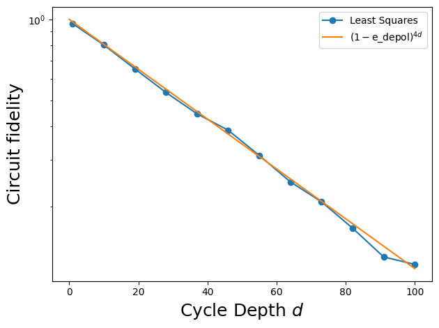
Fidelities
plt.plot(fids['cycle_depth'], fids['fidelity'], marker='o', label='Least Squares')

xx = np.linspace(0, fids['cycle_depth'].max())

# In XEB, we extract the depolarizing fidelity, which is
# related to (but not equal to) the Pauli error.
# For the latter, an error involves doing X, Y, or Z with E_PAULI/3
# but for the former, an error involves doing I, X, Y, or Z with e_depol/4
e_depol = E_PAULI / (1 - 1 / DIM**2)

# The additional factor of four in the exponent is because each layer
# involves two moments of two qubits (so each layer has four applications
# of a single-qubit single-moment depolarizing channel).
plt.plot(xx, (1 - e_depol) ** (4 * xx), label=r'$(1-\mathrm{e\_depol})^{4d}$')

plt.ylabel('Circuit fidelity', fontsize=18)
plt.xlabel('Cycle Depth $d$', fontsize=18)
plt.legend(loc='best')
plt.yscale('log')
plt.tight_layout()

from cirq.experiments.xeb_fitting import fit_exponential_decays

# Ordinarily, we'd use this function to fit curves for multiple pairs.
# We add our qubit pair as a column.
fids['pair'] = [(q0, q1)] * len(fids)

fit_df = fit_exponential_decays(fids)
fit_row = fit_df.iloc[0]
print(f"Noise model fidelity: {(1-e_depol)**4:.3e}")
print(f"XEB layer fidelity:   {fit_row['layer_fid']:.3e} +- {fit_row['layer_fid_std']:.2e}")
Noise model fidelity: 9.788e-01
XEB layer fidelity:   9.786e-01 +- 2.34e-04
