XEB calibration: Example and benchmark

This tutorial shows a detailed example and benchmark of XEB calibration, a calibration technique introduced in the Calibration: Overview and API tutorial.

Disclaimer: The data shown in this tutorial is exemplary and not representative of the QCS in production.

Setup

try:
    import cirq
except ImportError:
    !pip install --quiet cirq~=1.0.dev

# The Google Cloud Project id to use.
project_id = ""
processor_id = ""

from cirq_google.engine.qcs_notebook import get_qcs_objects_for_notebook
device_sampler = get_qcs_objects_for_notebook(project_id, processor_id)

if not device_sampler.signed_in:
    raise Exception("Please setup project_id in this cell or set the `GOOGLE_CLOUD_PROJECT` env var to your project id.")

import cirq
from cirq.experiments import random_quantum_circuit_generation as rqcg
import cirq_google as cg

import matplotlib.pyplot as plt
import numpy as np
import tqdm

Helper functions

from typing import Optional, Sequence


def create_random_circuit(
    qubits: Sequence[cirq.GridQubit],
    cycles: int,
    twoq_gate: cirq.Gate = cirq.FSimGate(np.pi / 4, 0.0),
    seed: Optional[int] = None,
) -> cirq.Circuit:
    return rqcg.random_rotations_between_grid_interaction_layers_circuit(
        qubits, 
        depth=cycles,
        two_qubit_op_factory=lambda a, b, _: twoq_gate.on(a, b),
        pattern=cirq.experiments.GRID_STAGGERED_PATTERN,
        single_qubit_gates=[cirq.PhasedXPowGate(phase_exponent=p, exponent=0.5)
                            for p in np.arange(-1.0, 1.0, 0.25)],
        seed=seed
    )



def create_loschmidt_echo_circuit(
    qubits: Sequence[cirq.GridQubit],
    cycles: int,
    twoq_gate: cirq.Gate = cirq.FSimGate(np.pi / 4, 0.0),
    seed: Optional[int] = None,
) -> cirq.Circuit:
    """Returns a Loschmidt echo circuit using a random unitary U.

    Args:
        qubits: Qubits to use.
        cycles: Depth of random rotations in the forward & reverse unitary.
        twoq_gate: Two-qubit gate to use.
        pause: Optional duration to pause for between U and U^\dagger.
        seed: Seed for circuit generation.
    """
    forward = create_random_circuit(qubits, cycles, twoq_gate, seed)
    return forward + cirq.inverse(forward) + cirq.measure(*qubits, key="z")



def to_ground_state_prob(result: cirq.Result) -> float:
    return np.mean(np.sum(result.measurements["z"], axis=1) == 0)

Select qubits

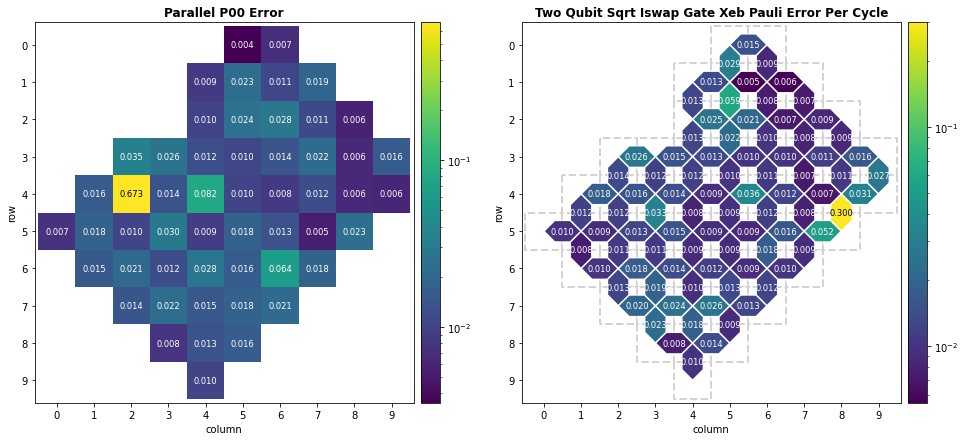
First we select a processor and calibration metric(s) to visualize the latest calibration report.

processor_id = ""
metrics = "parallel_p00_error, two_qubit_sqrt_iswap_gate_xeb_pauli_error_per_cycle"
metrics = [m.strip() for m in metrics.split(sep=",")]

from matplotlib.colors import LogNorm


_, axes = plt.subplots(
    nrows=1, ncols=len(metrics), figsize=(min(16, 8 * len(metrics)), 7)
)


calibration = cg.get_engine_calibration(processor_id=processor_id)
for i, metric in enumerate(metrics):
    calibration.heatmap(metric).plot(
        ax=axes[i] if len(metrics) > 1 else axes, 
        collection_options={"norm": LogNorm()}, 
        annotation_format="0.3f", 
        annotation_text_kwargs = {"size": "small"}
);

png

Using this report as a guide, we select a good set of qubits.

# Select qubit indices here.
qubit_indices = [
    (2, 5), (2, 6), (2, 7), (2, 8), (3, 8), 
    (3, 7), (3, 6), (3, 5), (4, 5), (4, 6)  
]
qubits = [cirq.GridQubit(*idx) for idx in qubit_indices]

An example random circuit on these qubits (used as the forward operations of the Loschmidt echo) is shown below.

create_random_circuit(qubits, cycles=10, seed=1)

Set up XEB calibration

Now we specify the cycle depths and other options for XEB calibration below. Note that all cirq.FSimGate parameters are characterized by default.

xeb_options = cg.LocalXEBPhasedFSimCalibrationOptions(
    cycle_depths=(5, 25, 50, 100),
    n_processes=1,
    fsim_options=cirq.experiments.XEBPhasedFSimCharacterizationOptions(
        characterize_theta=False,
        characterize_zeta=True,
        characterize_chi=True,
        characterize_gamma=True,
        characterize_phi=False,
    ),
)

Run a Loschmidt echo benchmark

"""Setup the Loschmidt echo experiment."""
cycle_values = range(0, 40 + 1, 4)
nreps = 20_000
trials = 10

sampler = cg.get_engine_sampler(
    project_id=project_id,
    processor_id=processor_id, 
    gate_set_name="sqrt_iswap",
)

loschmidt_echo_batch = [
    create_loschmidt_echo_circuit(qubits, cycles=c, seed=trial)
    for trial in range(trials) for c in cycle_values
]

Without calibration

First we run the Loschmidt echo without calibration.

# Run on the engine.
raw_results = sampler.run_batch(programs=loschmidt_echo_batch, repetitions=nreps)

# Convert measurements to survival probabilities.
raw_probs = np.array(
    [to_ground_state_prob(*res) for res in raw_results]
).reshape(trials, len(cycle_values))

With XEB calibration

Now we perform XEB calibration.

# Get characterization requests.
characterization_requests = cg.prepare_characterization_for_operations(loschmidt_echo_batch, xeb_options)

# Characterize the requests on the engine.
characterizations = cg.run_calibrations(characterization_requests, sampler)

# Make compensations to circuits in the Loschmidt echo batch.
xeb_calibrated_batch = [
    cg.make_zeta_chi_gamma_compensation_for_moments(circuit, characterizations).circuit
    for circuit in loschmidt_echo_batch
]

100%|██████████| 45/45 [00:46<00:00,  1.04s/it]
100%|██████████| 45/45 [01:50<00:00,  2.45s/it]
100%|██████████| 45/45 [01:00<00:00,  1.34s/it]
100%|██████████| 45/45 [02:24<00:00,  3.20s/it]

And run the XEB calibrated batch below.

# Run on the engine.
xeb_results = sampler.run_batch(programs=xeb_calibrated_batch, repetitions=nreps)

# Convert measurements to survival probabilities.
xeb_probs = np.array(
    [to_ground_state_prob(*res) for res in xeb_results]
).reshape(trials, len(cycle_values))

Compare results

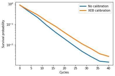
The next cell plots the results.

plt.semilogy(cycle_values, np.average(raw_probs, axis=0), lw=3, label="No calibration")
plt.semilogy(cycle_values, np.average(xeb_probs, axis=0), lw=3, label="XEB calibration")

plt.xlabel("Cycles")
plt.ylabel("Survival probability")
plt.legend();

png

A smaller (in magnitude) slope indicates lower two-qubit gate errors. You should see that XEB calibration produces lower errors than no calibration in the Loschmidt echo benchmark.