|
|
|
|
|
try:
    import cirq
except ImportError:
    print("installing cirq...")
    !pip install --quiet cirq
    print("installed cirq.")
This notebook demonstrates how to use the functionality in cirq.experiments to run parallel XEB end-to-end. "Parallel" means we characterize multiple pairs simultaneously.
import cirq
import numpy as np

%matplotlib inline
from matplotlib import pyplot as plt
Parallel XEB with library functions
The entire XEB workflow can be run by calling cirq.experiments.parallel_two_qubit_xeb and the combined single-qubit randomized benchmarking (RB) and XEB workflows can be run by calling cirq.experiments.run_rb_and_xeb.
# Simulation
qubits = cirq.GridQubit.rect(3, 2, 4, 3)
result = cirq.experiments.parallel_two_qubit_xeb(
    sampler=cirq.DensityMatrixSimulator(
        noise=cirq.depolarize(5e-3), dtype=np.complex128
    ),  # Any simulator or a ProcessorSampler.
    qubits=qubits,
)
100%|██████████| 243/243 [02:45<00:00, 1.47it/s]
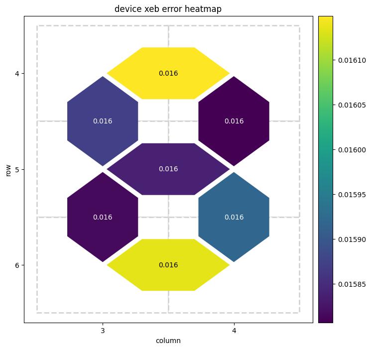
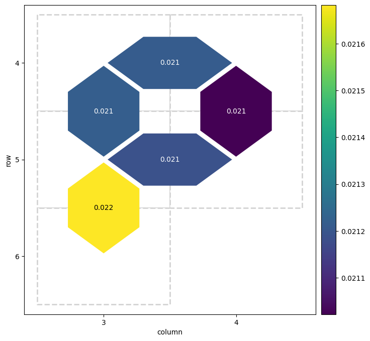
# The returned result is an instance of the `TwoQubitXEBResult` class which provides visualization methods like
result.plot_heatmap()
# plot the heatmap of XEB errors
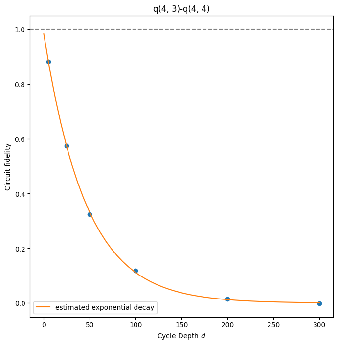
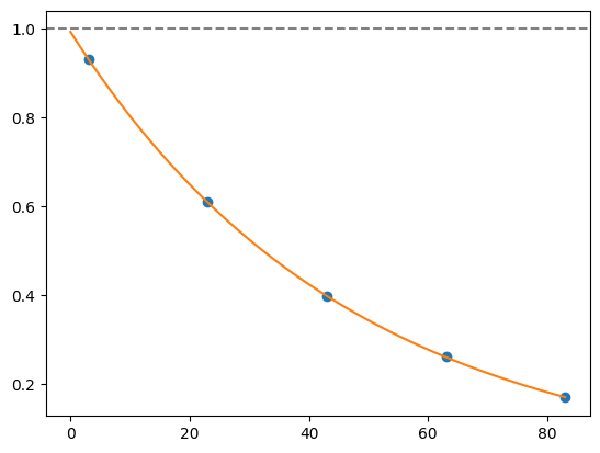
result.plot_fitted_exponential(*qubits[:2])
# plot the fitted model of xeb error of a qubit pair.
result.plot_histogram(); # plot a histogram of all xeb errors.
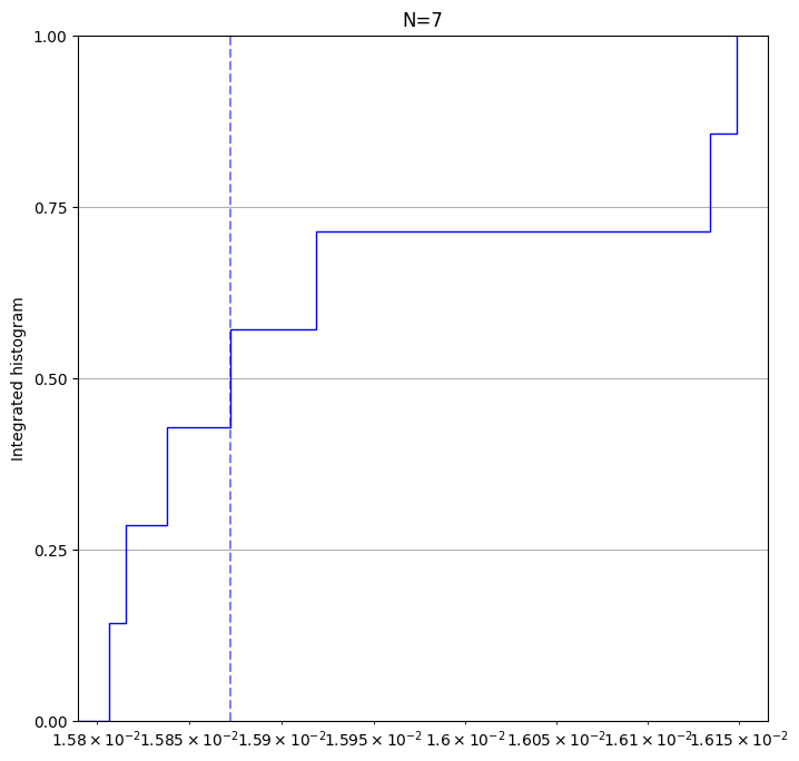
# `TwoQubitXEBResult` also has methods to retrieve errors.
print('pauli errors:', result.pauli_error())
print('xeb errors:', result.xeb_error(*qubits[:2]))
print('xeb fidelity:', result.xeb_fidelity(*qubits[:2]))
pauli errors: {(cirq.GridQubit(4, 3), cirq.GridQubit(4, 4)): np.float64(0.019835896750389596), (cirq.GridQubit(4, 3), cirq.GridQubit(5, 3)): np.float64(0.019613922392582306), (cirq.GridQubit(4, 4), cirq.GridQubit(5, 4)): np.float64(0.020158079809996406), (cirq.GridQubit(5, 3), cirq.GridQubit(5, 4)): np.float64(0.019523058811304374), (cirq.GridQubit(5, 3), cirq.GridQubit(6, 3)): np.float64(0.019736423224559763), (cirq.GridQubit(5, 4), cirq.GridQubit(6, 4)): np.float64(0.019596043847401635), (cirq.GridQubit(6, 3), cirq.GridQubit(6, 4)): np.float64(0.019928119059041058)}
xeb errors: 0.015868717400311705
xeb fidelity: 0.9841312825996883
The run_rb_and_xeb method returns an object of type InferredXEBResult which is like TwoQubitXEBResult except that it removes the single-qubit errors obtained from the single-qubit randomized benchmarking (RB) experiment to isolate the error from the two qubit gate.
Step by step XEB
The rest of this notebook explains how the parallel_two_qubit_xeb works internally. Note that the notebook uses SQRT_ISWAP as the entangling gate while parallel_two_qubit_xeb and run_rb_and_xeb default to CZ.
Set up Random Circuits
We create a library of 10 random, two-qubit circuits using the sqrt(ISWAP) gate. These library circuits will be mixed-and-matched among all the pairs on the device we aim to characterize.
from cirq.experiments import random_quantum_circuit_generation as rqcg

circuit_library = rqcg.generate_library_of_2q_circuits(
    n_library_circuits=20, two_qubit_gate=cirq.ISWAP**0.5, random_state=52
)
print(len(circuit_library))
20
# We will truncate to these lengths
max_depth = 100
cycle_depths = np.arange(3, max_depth, 20)
cycle_depths
array([ 3, 23, 43, 63, 83])
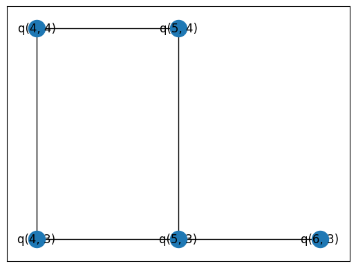
Determine the device topology
We will run on all pairs from a given device topology. Below, you can supply a device_name if you're authenticated to run on Google QCS. In that case, we will get the device object from the cloud endpoint and turn it into a graph of qubits. Otherwise, we mock a device graph by allocating arbitrary cirq.GridQubits to turn into a graph.
device_name = None  # change me!

import cirq.contrib.routing as ccr
import networkx as nx

if device_name is None:
    qubits = cirq.GridQubit.rect(3, 2, 4, 3)
    # Delete one qubit from the rectangular arangement to
    # 1) make it irregular 2) simplify simulation.
    qubits = qubits[:-1]
    sampler = cirq.DensityMatrixSimulator(noise=cirq.depolarize(5e-3))
    graph = ccr.gridqubits_to_graph_device(qubits)
else:
    import cirq_google as cg

    sampler = cg.get_engine_sampler(device_name, gate_set_name='sqrt_iswap')
    device = cg.get_engine_device(device_name)
    qubits = sorted(device.qubits)
    graph = ccr.gridqubits_to_graph_device(device.qubits)


pos = {q: (q.row, q.col) for q in qubits}
nx.draw_networkx(graph, pos=pos)
Set up our combinations
We take the library of two-qubit circuits in circuit_library and mix-and-match to sampled in parallel.
We will pass combs_by_layer and circuit_library to the sampling function which will "zip" the circuits according to these combinations. The outer list corresponds to the four cirq.GridInteractionLayers (one of four for the degree-four GridQubit-implied graph). The inner combinations matrix is a (n_combinations, n_pairs) ndarray of integers which index into the circuit library.
combs_by_layer = rqcg.get_random_combinations_for_device(
    n_library_circuits=len(circuit_library), n_combinations=10, device_graph=graph, random_state=53
)
combs_by_layer
[CircuitLibraryCombination(layer=cirq.experiments.GridInteractionLayer(col_offset=0, vertical=True, stagger=True), combinations=array([[ 5, 16],
        [12,  9],
        [ 5, 18],
        [11,  3],
        [ 6,  9],
        [13,  3],
        [11,  6],
        [14, 12],
        [16, 10],
        [18, 15]]), pairs=[(cirq.GridQubit(4, 4), cirq.GridQubit(5, 4)), (cirq.GridQubit(5, 3), cirq.GridQubit(6, 3))]),
 CircuitLibraryCombination(layer=cirq.experiments.GridInteractionLayer(col_offset=1, vertical=True, stagger=True), combinations=array([[16],
        [ 3],
        [12],
        [ 0],
        [ 5],
        [ 5],
        [ 0],
        [ 7],
        [ 9],
        [12]]), pairs=[(cirq.GridQubit(4, 3), cirq.GridQubit(5, 3))]),
 CircuitLibraryCombination(layer=cirq.experiments.GridInteractionLayer(col_offset=1, vertical=False, stagger=True), combinations=array([[13],
        [ 8],
        [ 8],
        [13],
        [ 1],
        [11],
        [11],
        [ 8],
        [14],
        [14]]), pairs=[(cirq.GridQubit(4, 3), cirq.GridQubit(4, 4))]),
 CircuitLibraryCombination(layer=cirq.experiments.GridInteractionLayer(col_offset=0, vertical=False, stagger=True), combinations=array([[18],
        [16],
        [ 2],
        [ 6],
        [ 1],
        [ 9],
        [11],
        [ 1],
        [ 9],
        [ 6]]), pairs=[(cirq.GridQubit(5, 3), cirq.GridQubit(5, 4))])]
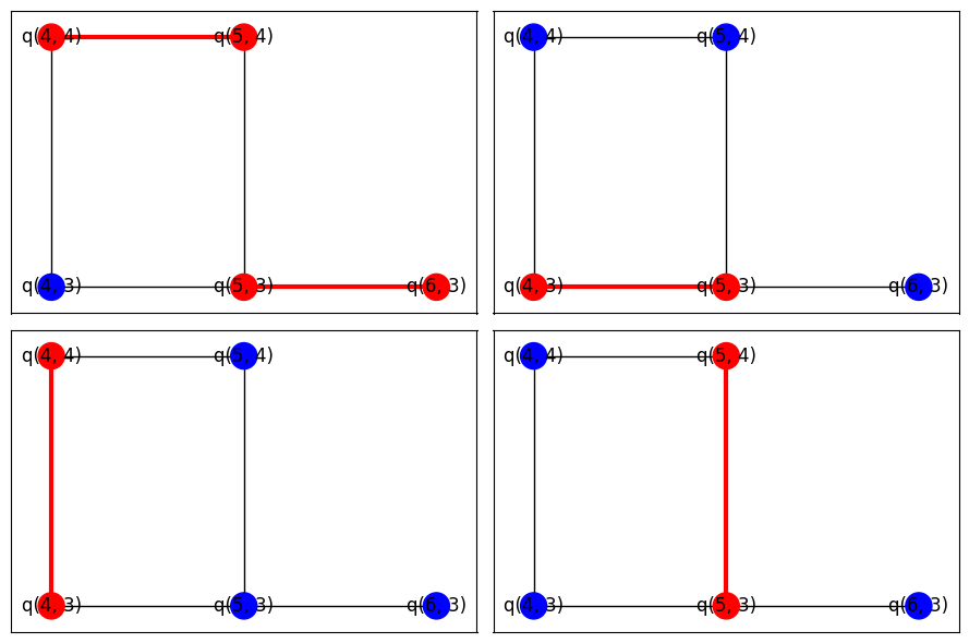
Visualize
Here, we draw the four layers' active pairs.
fig, axes = plt.subplots(2, 2, figsize=(9, 6))
for comb_layer, ax in zip(combs_by_layer, axes.reshape(-1)):
    active_qubits = np.array(comb_layer.pairs).reshape(-1)
    colors = ['red' if q in active_qubits else 'blue' for q in graph.nodes]
    nx.draw_networkx(graph, pos=pos, node_color=colors, ax=ax)
    nx.draw_networkx_edges(
        graph, pos=pos, edgelist=comb_layer.pairs, width=3, edge_color='red', ax=ax
    )

plt.tight_layout()
Take Data
The following call will execute the zipped circuits and sample bitstrings.
from cirq.experiments.xeb_sampling import sample_2q_xeb_circuits

sampled_df = sample_2q_xeb_circuits(
    sampler=sampler,
    circuits=circuit_library,
    cycle_depths=cycle_depths,
    combinations_by_layer=combs_by_layer,
    shuffle=np.random.RandomState(52),
    repetitions=10_000,
)
sampled_df
100%|██████████| 207/207 [00:45<00:00, 4.52it/s]
Benchmark Fidelities
from cirq.experiments.xeb_fitting import benchmark_2q_xeb_fidelities

fids = benchmark_2q_xeb_fidelities(
    sampled_df=sampled_df, circuits=circuit_library, cycle_depths=cycle_depths
)
fids
from cirq.experiments.xeb_fitting import fit_exponential_decays, exponential_decay

fidelities = fit_exponential_decays(fids)
heatmap_data = {}

for (_, _, pair), fidelity in fidelities.layer_fid.items():
    heatmap_data[pair] = 1.0 - fidelity

cirq.TwoQubitInteractionHeatmap(heatmap_data).plot();
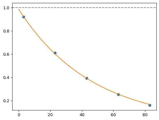
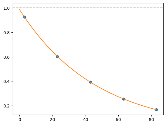
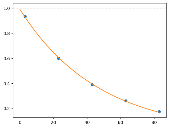
for i, record in fidelities.iterrows():
    plt.axhline(1, color='grey', ls='--')
    plt.plot(record['cycle_depths'], record['fidelities'], 'o')
    xx = np.linspace(0, np.max(record['cycle_depths']))
    plt.plot(xx, exponential_decay(xx, a=record['a'], layer_fid=record['layer_fid']))
    plt.show()

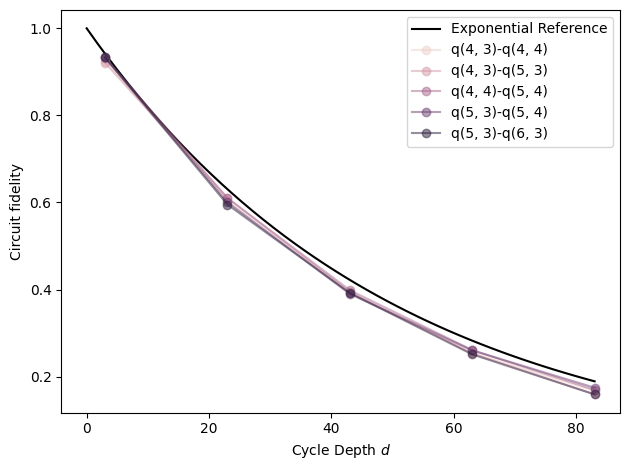
import seaborn as sns

# Give each pair its own color
colors = sns.cubehelix_palette(n_colors=graph.number_of_edges())
colors = dict(zip(graph.edges, colors))

# Exponential reference
xx = np.linspace(0, fids['cycle_depth'].max())
plt.plot(xx, (1 - 5e-3) ** (4 * xx), label=r'Exponential Reference', color='black')


# Plot each pair
def _p(fids):
    q0, q1 = fids.name
    plt.plot(
        fids['cycle_depth'],
        fids['fidelity'],
        'o-',
        label=f'{q0}-{q1}',
        color=colors[fids.name],
        alpha=0.5,
    )


fids.groupby('pair').apply(_p)

plt.ylabel('Circuit fidelity')
plt.xlabel('Cycle Depth $d$')
plt.legend(loc='best')
plt.tight_layout()
/tmpfs/tmp/ipykernel_78850/3110110171.py:25: DeprecationWarning: DataFrameGroupBy.apply operated on the grouping columns. This behavior is deprecated, and in a future version of pandas the grouping columns will be excluded from the operation. Either pass `include_groups=False` to exclude the groupings or explicitly select the grouping columns after groupby to silence this warning.
  fids.groupby('pair').apply(_p)
Optimize PhasedFSimGate parameters
We know what circuits we requested, and in this simulated example, we know what coherent error has happened. But in a real experiment, there is likely unknown coherent error that you would like to characterize. Therefore, we make the five angles in PhasedFSimGate free parameters and use a classical optimizer to find which set of parameters best describes the data we collected from the noisy simulator (or device, if this was a real experiment).
import multiprocessing

pool = multiprocessing.get_context('spawn').Pool()
from cirq.experiments.xeb_fitting import (
    parameterize_circuit,
    characterize_phased_fsim_parameters_with_xeb_by_pair,
    SqrtISwapXEBOptions,
)

# Set which angles we want to characterize (all)
options = SqrtISwapXEBOptions(
    characterize_theta=True,
    characterize_zeta=True,
    characterize_chi=True,
    characterize_gamma=True,
    characterize_phi=True,
)
# Parameterize the sqrt(iswap)s in our circuit library
pcircuits = [parameterize_circuit(circuit, options) for circuit in circuit_library]

# Run the characterization loop
characterization_result = characterize_phased_fsim_parameters_with_xeb_by_pair(
    sampled_df,
    pcircuits,
    cycle_depths,
    options,
    pool=pool,
    # ease tolerance so it converges faster:
    fatol=1e-2,
    xatol=1e-2,
)
characterization_result.final_params
{(cirq.GridQubit(5, 3),
  cirq.GridQubit(5, 4)): {'theta': np.float64(-0.8367987404054755), 'zeta': np.float64(0.10041558244274296), 'chi': np.float64(-0.07510134699446311), 'gamma': np.float64(-0.017183029157944202), 'phi': np.float64(0.004193753360909505)},
 (cirq.GridQubit(4, 3),
  cirq.GridQubit(4, 4)): {'theta': np.float64(-0.8474371212531532), 'zeta': np.float64(-0.10035248634877036), 'chi': np.float64(-0.07034612478660182), 'gamma': np.float64(0.050899749487735915), 'phi': np.float64(-0.041682247860173494)},
 (cirq.GridQubit(4, 3),
  cirq.GridQubit(5, 3)): {'theta': np.float64(-0.7552448278453846), 'zeta': np.float64(0.033253969974588855), 'chi': np.float64(-0.03479666867301002), 'gamma': np.float64(0.03136281359839602), 'phi': np.float64(-0.06806601866053645)},
 (cirq.GridQubit(4, 4),
  cirq.GridQubit(5, 4)): {'theta': np.float64(-0.7790601994013041), 'zeta': np.float64(0.032579693881346745), 'chi': np.float64(-0.02279511443835067), 'gamma': np.float64(0.00337801077356593), 'phi': np.float64(0.0352923155799907)},
 (cirq.GridQubit(5, 3),
  cirq.GridQubit(6, 3)): {'theta': np.float64(-0.758190997670132), 'zeta': np.float64(0.004304546463840975), 'chi': np.float64(-0.049149081691340135), 'gamma': np.float64(0.0020049245053540667), 'phi': np.float64(0.025945488060518777)} }
characterization_result.fidelities_df
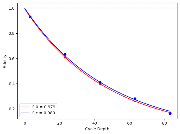
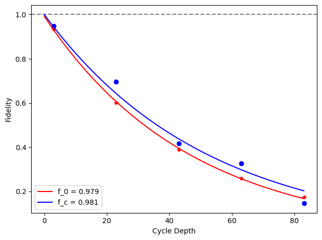
from cirq.experiments.xeb_fitting import before_and_after_characterization

before_after_df = before_and_after_characterization(fids, characterization_result)
before_after_df
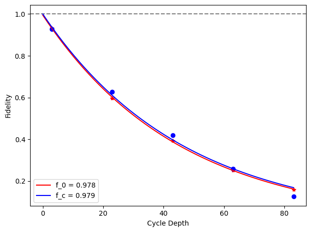
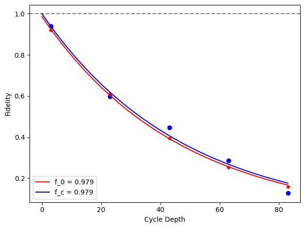
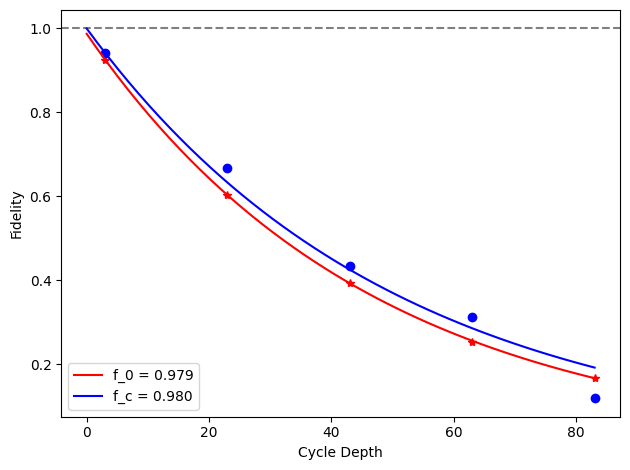
for i, row in before_after_df.iterrows():
    plt.axhline(1, color='grey', ls='--')
    plt.plot(row['cycle_depths_0'], row['fidelities_0'], '*', color='red')
    plt.plot(row['cycle_depths_c'], row['fidelities_c'], 'o', color='blue')

    xx = np.linspace(0, np.max(row['cycle_depths_0']))
    plt.plot(
        xx,
        exponential_decay(xx, a=row['a_0'], layer_fid=row['layer_fid_0']),
        color='red',
        label=f'f_0 = {row["layer_fid_0"]:.3f}',
    )
    plt.plot(
        xx,
        exponential_decay(xx, a=row['a_c'], layer_fid=row['layer_fid_c']),
        color='blue',
        label=f'f_c = {row["layer_fid_c"]:.3f}',
    )

    plt.xlabel('Cycle Depth')
    plt.ylabel('Fidelity')
    plt.legend(loc='best')
    plt.tight_layout()
    plt.show()