
|
|
|
|
|
This notebook shows how to simulate the one-dimensional Fermi-Hubbard Hamiltonian
\[ H = - J \sum_{j = 1}^{L - 1} \sum_{\sigma \in \{ \uparrow, \downarrow \} } c_{j, \sigma}^\dagger c_{j + 1, \sigma} + \text{h.c.} + U \sum_{j} n_{j\uparrow} n_{j\downarrow} \]
using FQE. Here \(j = 1, ..., L\) denotes site/orbital and \(\sigma \in \{ \uparrow, \downarrow \}\) denotes spin. By the end of the tutorial, we reproduce plots from the Fermi-Hubbard experiment paper and the corresponding ReCirq tutorial.
try:
    import fqe
except ImportError:
    # TODO: Change to `pip install fqe --quiet` when FQE>0.1.0 is released.
    !pip install git+https://github.com/quantumlib/OpenFermion-FQE --quiet
import copy
from itertools import product

import matplotlib.pyplot as plt
import numpy as np
from scipy import sparse
from scipy.linalg import expm

import openfermion as of
import fqe
Defining the Hamiltonian
We first define the Fermi-Hubbard Hamiltonian using OpenFermion.
"""Define the Hamiltonian."""
# Parameters.
nsites = 4
U = 2.0
J = -1.0

hubbard = of.fermi_hubbard(1, nsites, tunneling=-J, coulomb=U, periodic=False)
Time evolution
In this section we show how to do time evolution with FQE. We start from a random initial state in the two-particle \(S_z = 0\) sector to ignore the details of state preparation in the Fermi-Hubbard experiment paper for now.
nele, sz = 2, 0
init_wfn = fqe.Wavefunction([[nele, sz, nsites]])
init_wfn.set_wfn(strategy="random")
To do the time evolution, we can simply call the fqe.Wavefunction.time_evolve method with the Hubbard Hamiltonian and evolution time. When passing time_evolve a general fermion operator, FQE converts this into a dense Hamiltonian for time evolution. The evolution is accomplished by a Taylor expansion method.
%%time
e_time = 0.9
true_evolved_fqe = init_wfn.time_evolve(e_time, hubbard)
CPU times: user 92.4 ms, sys: 0 ns, total: 92.4 ms
Wall time: 23.3 ms
We can compare the speed of this method to direct matrix exponentiation as follows.
%%time
# Convert FQE wavefunction to an 2^n vector |𝛹⟩.
init_cirq_wfn = fqe.to_cirq(init_wfn)

# Exponentiate the (sparse) Hamiltonian U = exp(-i H t).
unitary = expm(-1j * e_time * of.get_sparse_operator(hubbard).todense())

# Do the time evolution |𝛹'⟩ = U |𝛹⟩.
true_evolved_cirq = unitary @ init_cirq_wfn
CPU times: user 558 ms, sys: 17.7 ms, total: 576 ms
Wall time: 168 ms
The next cell verifies both methods produce the same final wavefunction.
fidelity = abs(fqe.vdot(true_evolved_fqe, fqe.from_cirq(true_evolved_cirq, thresh=1e-12)))**2
assert np.isclose(fidelity, 1.0)
Even for a small number of sites, the FQE simulation is notably faster than the direct matrix exponentian simulation. This is because FQE evolves in only fixed particle and spin subspace and because the time evolution is simulated by series expansion of the matrix exponent.
Trotterization
We can apply the Trotter formula and evolve the hopping Hamiltonian (one-body terms)
\[ H_{\text{hop} } := - J \sum_{j = 1}^{L - 1} \sum_{\sigma \in \{ \uparrow, \downarrow \} } c_{j, \sigma}^\dagger c_{j + 1, \sigma} + \text{h.c.} \]
and the charge-charge interaction (two-body terms)
\[ H_{\text{cc} } := U \sum_{j} n_{j\uparrow} n_{j\downarrow} \]
separately for short time steps. We first split up the Hamiltonian into one-body and two-body terms.
# Each site has two spins.
nqubits = 2 * nsites

# One-body (hopping) terms.
one_body_terms = [
    op + of.hermitian_conjugated(op) for op in (
        of.FermionOperator(((i, 1), (i + 2, 0)), coefficient=J) for i in range(nqubits - 2)
    )
]

# Two-body (charge-charge) terms.
two_body_terms = [
    of.FermionOperator(((i, 1), (i, 0), (i + 1, 1), (i + 1, 0)), coefficient=U)
    for i in range(0, nqubits, 2)
]

# Verify this produces the same Hamiltonian from OpenFermion.
assert sum(one_body_terms) + sum(two_body_terms) == hubbard
The Hopping Hamiltonian is a \(2^n \times 2^n\) matrix, so one method for time evolution is directly exponentiating this matrix to apply \(e^{- i t H_{\text{hop} } }\) to the initial state.
# Get the 2^n x 2^n matrix (as a sparse operator).
sparse_hopping_matrix = of.get_sparse_operator(sum(one_body_terms))

# Exponentiate the matrix.
unitary = expm(-1j * e_time * sparse_hopping_matrix.todense())

# Time-evolve the initial state.
evolved_cirq_wfn = unitary @ init_cirq_wfn
Now let's see how to do this in FQE. We first recognize the hopping Hamiltonian can be written as the following \(n \times n\) matrix.
hopping_matrix = J * (np.diag([1] * (nsites - 1), k=1) + np.diag([1] * (nsites - 1), k=-1))
print(hopping_matrix)
[[-0. -1. -0. -0.]
 [-1. -0. -1. -0.]
 [-0. -1. -0. -1.]
 [-0. -0. -1. -0.]]
Using the unitary generated by this matrix, we can evolve the initial state using the function evolve_fqe_givens as shown below.
from fqe.algorithm.low_rank import evolve_fqe_givens

umat = expm(-1j * e_time * hopping_matrix)
evolved_wfn = evolve_fqe_givens(init_wfn, umat)
We can verify the wavefunction evolved by FQE and the wavefunction evolved by direct matrix exponentiation are identical.
fidelity = abs(fqe.vdot(evolved_wfn, fqe.from_cirq(evolved_cirq_wfn, thresh=1e-6)))**2
assert np.isclose(fidelity, 1.0)
Like the Hopping Hamiltonian, the charge-charge interaction is a \(2^n \times 2^n\) matrix, so we can again apply \(e^{- i t H_{\text{cc} } }\) to the initial state.
# Get the 2^n x 2^n matrix (as a sparse operator).
sparse_charge_charge_matrix = of.get_sparse_operator(sum(two_body_terms))

# Exponentiate the matrix.
unitary = expm(-1j * e_time * sparse_charge_charge_matrix.todense())

# Time-evolve the initial state.
evolved_cirq_wfn = unitary @ init_cirq_wfn
As with the hopping Hamiltonian, the charge-charge term can be written as an \(n \times n\) matrix as follows.
charge_charge_matrix = np.diag([U] * nsites)
charge_charge_matrix
array([[2., 0., 0., 0.],
       [0., 2., 0., 0.],
       [0., 0., 2., 0.],
       [0., 0., 0., 2.]])
We use this to perform time-evolution with the evolve_fqe_charge_charge_alpha_beta function. This function applies
\[ \exp\left(-i t \sum_{i,j} v_{i, j} n_{i, \alpha} n_{j, \beta} \right) \]
for any coefficients \(v_{i, j}\) to the wavefunction. (One can easiliy check the charge-charge interaction \(H_{\text{cc} }\) can be written in this way.)
from fqe.algorithm.low_rank import evolve_fqe_charge_charge_alpha_beta

evolved_fqe_wfn = evolve_fqe_charge_charge_alpha_beta(
    init_wfn,
    charge_charge_matrix,
    e_time
)
As before we can verify this produces the same evolved wavefunction as direct matrix exponentiation.
fidelity = abs(fqe.vdot(evolved_fqe_wfn, fqe.from_cirq(evolved_cirq_wfn, thresh=1e-6)))**2
assert np.isclose(fidelity, 1.0)
At this point we can simulate a specified number of Trotter steps as follows.
# Set the number of Trotter steps.
trotter_steps = 10

# Evolution under the hopping Hamiltonian for a single Trotter step.
umat = expm(-1j * hopping_matrix * (e_time / trotter_steps))

# Simulate each Trotter step.
current_wfn = copy.deepcopy(init_wfn)
for _ in range(trotter_steps):
    # Evolve the Hopping Hamiltonian.
    current_wfn = evolve_fqe_givens(current_wfn,  u=umat)

    # Evolve the charge-charge interaction.
    current_wfn = evolve_fqe_charge_charge_alpha_beta(
        current_wfn,
        charge_charge_matrix,
        e_time / trotter_steps,
    )
Since we already evolved the wavefunction without Trotterization, we can compare the Trotterized evolution to this below.
trotterized_fidelity = abs(fqe.vdot(true_evolved_fqe, current_wfn))**2
print("Trotterized fidelity:", trotterized_fidelity)
Trotterized fidelity: 0.9983245612277033
One can increase the number of Trotter steps to increase this fidelity. When reproducing experimental results below, we will use Trotterization as in the paper.
Reproducing experimental results
We now reproduce results from the Fermi-Hubbard experiment paper using the time-evolution methods in FQE we have discussed above. The only remaining ingredient is the initial state.
Preparing the initial state
The initial state in the Fermi-Hubbard experiment is the ground state of a non-interacting Hamiltonian with different onsite potentials. The spin-up sector and spin-down sector have no coupling. We create the two non-interacting components of this Hamiltonian below.
# Parameters used in the Fermi-Hubbard experiment.
nsites = 8
l_up = 4
m_up = 4.5
sigma_up = 1

# For convenience.
site_index = np.arange(1, nsites + 1)

# Creating the spin-up and spin-down Hamiltonians.
spin_up_ham = np.diag([-1.] * (nsites - 1), k=1) + np.diag([-1.] * (nsites - 1), k=-1)
spin_up_ham += np.diag(-l_up * np.exp(-0.5 * (site_index - m_up)**2) / sigma_up**2)
spin_down_ham = np.diag([-1.] * (nsites - 1), k=1) + np.diag([-1.] * (nsites - 1), k=-1)
We know our one-body Hamiltonian is diagonalized by a quadratic Hamiltonian that can be implemented via a Givens rotation network. We now occupy the two lowest states \(b^\dagger_{1a} b^\dagger_{2a} b^\dagger_{1b} b^\dagger_{2b}|\text{vac}\rangle\) and then reverse-transform back to the original basis.
# Initialize wavefunction to occupy the two lowest states.
init_wfn = fqe.Wavefunction([[nsites // 2, 0, nsites]])
init_wfn.set_wfn(strategy='hartree-fock')
init_wfn.print_wfn()
Sector N = 4 : S_z = 0
a'00000011'b'00000011' (1+0j)
To transform back, we first diagonalize the spin-up and spin-down hamiltonians to get the eigenbasis.
_, v_up = np.linalg.eigh(spin_up_ham)
_, v_down = np.linalg.eigh(spin_down_ham)
And now rotate back to the original basis through a one-body transform implemented with the Givens rotation network.
from fqe.algorithm.low_rank import evolve_fqe_givens_sector


init_wfn = evolve_fqe_givens_sector(init_wfn, v_up, sector='alpha')
init_wfn = evolve_fqe_givens_sector(init_wfn, v_down, sector='beta')
Now that we have the initial state, we can compute the charge (\(+\)) and spin (\(-\)) density, respectively
\[ \rho_{j}^{\pm} = \langle n_{j, \uparrow} \rangle \pm \langle n_{j, \downarrow} \rangle, \]
at time \(t = 0\).
Plotting.
plt.rcParams['font.family'] = 'sans-serif'
plt.rcParams['font.size'] = 14
colors = ['#4285F4', '#EA4335']

# Plot the data.
opdm_a, opdm_b = init_wfn.sector((nsites // 2, 0)).get_spin_opdm()
charge_density = np.diagonal(opdm_a).real + np.diagonal(opdm_b).real
spin_density = np.diagonal(opdm_a).real - np.diagonal(opdm_b).real

fig, ax = plt.subplots(nrows=1, ncols=1, figsize=(6, 4))
plt.plot(site_index, charge_density, "-o", color=colors[0], label="Charge")
plt.plot(site_index, spin_density, "-o", color=colors[1], label="Spin")

# Axes.
ax.set_ylabel(r"Charge density $\rho^+$", color=colors[0])
ax_twin = ax.twinx()
ax_twin.set_ylabel(r"Spin density $\rho^-$", color=colors[1])

ax.set_xticks(site_index)
ax.set_xlabel("Site index")
ax.legend();
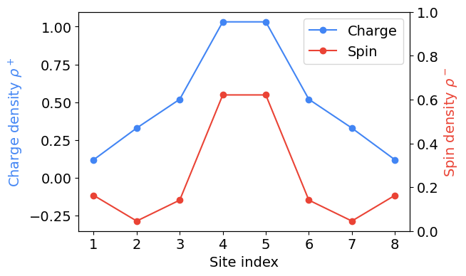
One can check this plot reproduces Fig. 2(a) from the Fermi-Hubbard experiment paper.
Compare to direct diagonalization
Here we quickly compare our previous procedure for creating the initial state to exact diagonalization. We will see they are identical.
The cell below creates the initial non-interacting Hamiltonian to diagonalize in two steps.
# (1) Create Fermion operator.
h0 = np.zeros((2 * nsites, 2 * nsites))
h0[::2, ::2] = spin_up_ham
h0[1::2, 1::2] = spin_down_ham

fop = of.FermionOperator()
for p, q in product(range(2 * nsites), repeat=2):
    fop += of.FermionOperator(((p, 1), (q, 0)), coefficient=h0[p, q])

fop_mat = of.get_sparse_operator(fop)

# (2) Project Fermion operator.
dim = 2**(2 * nsites)
diag_val = []
diag_pos = []

for ii in range(dim):
    ket = np.binary_repr(ii, width=2*nsites)
    ket_a = list(map(int, ket[::2]))
    ket_b = list(map(int, ket[1::2]))

    if np.isclose(sum(ket_a) + sum(ket_b), 4) and np.isclose(sum(ket_a) - sum(ket_b), 0):
        assert np.isclose(sum(ket_a), 2)
        assert np.isclose(sum(ket_b), 2)
        diag_val.append(1)
        diag_pos.append(ii)


proj_n = sparse.coo_matrix((diag_val, (diag_pos, diag_pos)), shape=(dim, dim))
fop_mat = proj_n @ fop_mat @ proj_n  # Hamiltonian to diagonalize.
Now that we have the Hamiltonian, we can diagonalize it to get the ground state.
evals, evecs = sparse.linalg.eigsh(fop_mat.real, k=1)
At this point we have the initial wavefunction as a \(2^n\) element vector. Below we convert this to the FQE representation and check it is identical to the previous initial wavefunction we prepared.
init_wfn_from_diag = fqe.from_cirq(evecs[:, 0].flatten(), thresh=1.0E-12)

# Check.
fidelity = abs(fqe.vdot(init_wfn, init_wfn_from_diag)) ** 2
assert np.isclose(fidelity, 1.0)
Computing the time-evolved charge and spin density
We now time-evolve the initial state under the Fermi-Hubbard model. As in the paper, we use time step \(\tau = 0.3 \hbar / J\) for a total simulation time of \(16.5 \hbar / J\). (Note that we use atomic units where \(\hbar = 1\).)
# Set the time step and number of Trotter steps (using hbar = 1).
dt = 0.3
trotter_steps = 55

hopping_u = expm(-1j * dt * spin_down_ham)
charge_u = np.diag([U] * nsites)

opdms_alpha = [opdm_a]
opdms_beta = [opdm_b]
real_times = [0.0]

current_time = 0.0
final_wfn = init_wfn
for tt in range(trotter_steps):
    final_wfn = evolve_fqe_givens(final_wfn, hopping_u)
    final_wfn = evolve_fqe_charge_charge_alpha_beta(final_wfn, charge_u, dt)
    current_time += dt
    opdm_a_current, opdm_b_current = final_wfn.sector((nsites // 2, 0)).get_spin_opdm()

    # Store the opdms at each time step.
    opdms_alpha.append(opdm_a_current)
    opdms_beta.append(opdm_b_current)
    real_times.append(current_time)
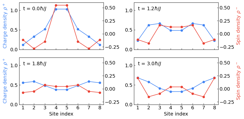
Using the stored data, we compute the charge and spin density at various times below.
# Times to plot the charge & spin density at.
times = [0.0, 1.2, 1.8, 3.0]
time_indices = [int(t / dt) for t in times]

charge_densities = []
spin_densities = []
for idx in time_indices:
    charge_densities.append(np.diagonal(opdms_alpha[idx] + opdms_beta[idx]).real)
    spin_densities.append(np.diagonal(opdms_alpha[idx] - opdms_beta[idx]).real)
We now plot these values to reproduce Fig. 1(a) from the Fermi-Hubbard paper.
Plotting.
fig, axes = plt.subplots(nrows=2, ncols=2, figsize=(10, 5), sharex=True)

for (i, ax) in enumerate(axes.flatten()):
    ax.plot(site_index, charge_densities[i], "-o", color=colors[0])
    ax_twin = ax.twinx()
    ax_twin.plot(site_index, spin_densities[i], "-o", color=colors[1])

    ax.set_ylim([0, 1.2])
    ax_twin.set_ylim([-0.3, 0.6])
    ax.tick_params(which="both", direction="in")
    ax_twin.tick_params(which="both", direction="in")

    if i >= 2:
        ax.set_xlabel("Site index")
    if i % 2 == 0:
        ax.set_ylabel(r"Charge density $\rho^+$", color=colors[0])
    if i % 2 == 1:
        ax_twin.set_ylabel(r"Spin density $\rho^-$", color=colors[1])
    ax.text(1, 1, rf"t = ${times[i]} \hbar / J$")

plt.xticks(site_index)
plt.tight_layout()
plt.show();
Computing the charge and spin spread
Last, we use this data to compute the charge and spin spread.
charge_spread = []
spin_spread = []
spread_func = np.abs(np.arange(1, nsites + 1) - (nsites + 1) / 2)

for ii in range(len(opdms_alpha)):
    charge_spread.append(np.sum(np.multiply(spread_func, np.diagonal(opdms_alpha[ii] + opdms_beta[ii]).real)))
    spin_spread.append(np.sum(np.multiply(spread_func, np.diagonal(opdms_alpha[ii] - opdms_beta[ii]).real)))
Plotting.
fig, ax = plt.subplots(nrows=1, ncols=1)

stop = 11
ax.plot(real_times[:stop], charge_spread[:stop], "-o", color=colors[0])
axtwin = ax.twinx()
axtwin.plot(real_times[:stop], spin_spread[:stop], "-o", color=colors[1])

ax.set_ylim([5, 10])
axtwin.set_ylim([-2.5, 2.6]);

ax.set_xticks(real_times[:stop])

ax.set_xlabel(r"Time $(\hbar / J)$")
ax.set_ylabel(r"Charge spread $\kappa^+$", color=colors[0])
axtwin.set_ylabel(r"Spin spread $\kappa^-$", color=colors[1]);
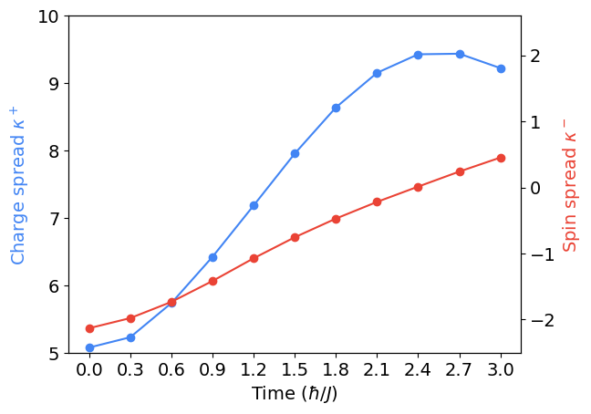
One can check this reproduces the \(u = 0\) subplot from Fig. 2(b) in the Fermi-Hubbard paper.