
|
|
|
|
|
This notebook demonstrates how to define, execute, and plot the results of a single instance of the Fermi-Hubbard experiment. We show how to run the experiment using a Cirq simulator and a quantum processor through Google's Quantum Computing Service.
The Fermi-Hubbard model on a one-dimensional lattice of \(L\) sites with open boundary conditions is defined by the Hamiltonian
\[ H = - J \sum_{j = 1}^{L - 1} \sum_{\nu = \uparrow, \downarrow} c_{j, \nu}^\dagger c_{j + 1, \nu} + \text{h.c.} + U \sum_{j = 1}^{L} n_{j, \uparrow} n_{j, \downarrow} + \sum_{j = 1}^{L} \sum_{\nu = \uparrow, \downarrow} \epsilon_{j, \nu} n_{j, \nu} \]
where \(c_{j, \nu}\) (\(c_{j, \nu}^\dagger\)) are the fermionic annihilation (creation) operators associated to site number \(j\) and spin state \(\nu\), and \(n_{j, \nu} = c_{j, \nu}^\dagger c_{j, \nu}\) are the number operators. The hopping term with coefficient \(J\) describes particles tunneling between neighboring sites, the onsite interaction term with coefficient \(U\) introduces an energy difference for doubly occupied sites, and the term \(\epsilon_{j, \nu}\) represents spin-dependent local potentials.
Our goal in this experiment is to compute the charge and spin densities which are defined as the sum and difference of the spin-up and spin-down particle densities, respectively
\[ \rho_{j}^{\pm} = \langle n_{j, \uparrow} \rangle \pm \langle n_{j, \downarrow} \rangle, \]
after simulating the Fermi-Hubbard model for some evolution time. Here, the expectation is taken with respect to the extended Hamiltonian
\[ H' = H + V \sum_{j = 1}^{L - 1} \sum_{\nu = \uparrow, \downarrow} n_{j, \nu} n_{j + 1, \nu} \]
which has an additional interaction term between neighboring fermionic sites. This enables extended simulations beyond the standard Fermi-Hubbard model.
Setup
We first install ReCirq which contains code for running Fermi-Hubbard experiments.
try:
    import recirq
except ImportError:
    print("Installing ReCirq...")
    !pip install git+https://github.com/quantumlib/recirq --quiet
    print("Installed ReCirq!")
To track the progress of simulating experiments, we use the tqdm package.
try:
    import ipywidgets
except ImportError:
    !pip install ipywidgets --quiet
    !jupyter nbextension enable --py widgetsnbextension --sys-prefix
We can now import Cirq and the fermi_hubbard module from ReCirq.
import cirq

from recirq import fermi_hubbard
from recirq.fermi_hubbard import publication

# Hide numpy warnings
import warnings
warnings.filterwarnings("ignore")
Experiment parameters
The first step is to decide on exact experiment parameters including problem Hamiltonian, initial state description, as well as a mapping from fermions to qubits on the device. Once we have this information, we can create circuits and run the experiment.
Qubit layout
We will simulate the Fermi-Hubbard model on \(L = 8\) sites. Each site is represented by two qubits due to the two spin states, so we need a total of \(16\) qubits to simulate the experiment.
The function rainbow23_layouts returns a set of \(16\)-qubit subgrids of the Google Rainbow processor.
"""Get all layouts for 8 sites on a 23-qubit subgrid of the Google Rainbow processor."""
layouts = publication.rainbow23_layouts(sites_count=8)
print(f"There are {len(layouts)} total qubit layouts.")
There are 16 total qubit layouts.
We can see an example layout by printing out its text diagram.
"""Display an example layout."""
print(layouts[0].text_diagram())
1↓ q(4, 1)━━━1↑ q(4, 2)
│            │
│            │
2↓ q(5, 1)━━━2↑ q(5, 2)───3↑ q(5, 3)
│                         │
│                         │
3↓ q(6, 1)───4↓ q(6, 2)━━━4↑ q(6, 3)───5↑ q(6, 4)
             │                         │
             │                         │
             5↓ q(7, 2)───6↓ q(7, 3)━━━6↑ q(7, 4)───7↑ q(7, 5)
                          │                         │
                          │                         │
                          7↓ q(8, 3)───8↓ q(8, 4)━━━8↑ q(8, 5)
The layout indicates the site index \(j\) and spin state \(\nu\), as well as which cirq.GridQubit on the Rainbow processor this combination of \((j, \nu)\) is encoded into. One can choose a different layout in the previous cell to see how the configurations vary.
Problem parameters
Let's use the Hamiltonian with uniform \(J = 1\) and \(U = 2\) on each site, initial state prepared as a ground state of a non-interacting Hamiltonian with trapping potential of a Gaussian shape, Trotter step size equal to 0.3, and two particles per chain. The problem parameters with this initial state can be prepared with the pre-defined function trapping_instance.
"""Get FermiHubbardParameters (problem descriptions) for each qubit layout with the above parameters."""
parameters = [
    publication.trapping_instance(
        layout, u=2, dt=0.3, up_particles=2, down_particles=2
    )
    for layout in layouts
]
Other configurations which support site-dependent \(U\) and \(J\) coefficients can be prepared by creating instances of the
fermi_hubbard.FermiHubbardParametersdata class explicitly.
The results are instances of the FermiHubbardParameters data class for each layout. This data class uniquely defines the configuration to run and contains information such as the Hamiltonian, initial state, layout, and time step. Below, we display these values for an example element of parameters.
"""Display the Hamiltonian for an example problem description."""
parameters_example = parameters[0]
print(parameters_example.hamiltonian)
Hamiltonian(sites_count=8, j=1.0, u=2, v=0, local_charge=0, local_spin=0, mu_up=0, mu_down=0)
We can also see the initial state:
parameters_example.initial_state
IndependentChainsInitialState(up=GaussianTrappingPotential(particles=2, center=0.5, sigma=0.14285714285714285, scale=-4), down=UniformTrappingPotential(particles=2))
And the time step:
parameters_example.dt
0.3
Circuits
One can directly run an experiment from a FermiHubbardParameters instance (which we will do in the next section). However, it is illustrative to construct the circuits to see how the Fermi-Hubbard execution works.
Circuit creation
To create a circuit from a description of a problem, the function fermi_hubbard.create_circuits can be used. This function inputs a FermiHubbardParameters instance (i.e., a problem description) and number of Trotter steps. It returns circuits for constructing the initial state, simulating time-evolution via a number of Trotter steps, and measuring to compute observables.
"""Create circuits from a problem description."""
initial, trotter, measurement = fermi_hubbard.create_circuits(parameters_example, trotter_steps=1)
Below, we display the complete circuit to execute which is a sum of the three component circuits above.
"""Display the total circuit to execute."""
circuit = initial + trotter + measurement
circuit
Circuit decomposition
The circuit above is constructed using gates which are not native to Google hardware, for example cirq.FSim or cirq.CZ with arbitrary exponent. To run these circuits on Google hardware, we have to convert them into native operations. For the Fermi-Hubbard experiment, a special converter called ConvertToNonUniformSqrtIswapGates is provided.
This converter has the ability to decompose gates to \(\sqrt{\small \mbox{iSWAP} }\) both perfectly (i.e., without noise) and with unitary parameters deviating from the perfect ones and varying between qubit pairs. The function ideal_sqrt_iswap_converter creates an instance of the noiseless converter which decomposes \(\sqrt{\small \mbox{iSWAP} }\) gates exactly as cirq.FSim(π/4, 0). The function google_sqrt_iswap_converter creates an instance of the noisy converter which approximates the average values on Rainbow processor (which are about cirq.FSim(π/4, π/24) on each two-qubit pair).
Below we show an example of the perfect decomposition into the \(\sqrt{\small \mbox{iSWAP} }\) gate set.
"""Convert the circuit to native hardware gates perfectly (without noise)."""
publication.ideal_sqrt_iswap_converter().convert(circuit)
We will consider both ideal and noisy decompositions when executing the experiment below.
Cirq simulation
This section demonstrates how to simulate experiments using Cirq simulator. We will simulate the evolution from \(0\) to \(10\) Trotter steps. Physically, this corresponds to an evolution time of \(t = 3 \hbar / J\).
"""Set the number of Trotter steps to simulate."""
trotter_steps = range(10 + 1)
Ideal
As mentioned above, we can use the ideal_sqrt_iswap_converter to convert circuits perfectly into the \(\sqrt{\small \mbox{iSWAP} }\) gate set. The Fermi-Hubbard project provides ConvertingSampler that converts circuits before executing ands sampling from them. We get an ideal sampler below.
"""Get an ideal sampler to simulate experiments."""
ideal_sampler = fermi_hubbard.ConvertingSampler(
    cirq.Simulator(), publication.ideal_sqrt_iswap_converter().convert
)
We can now run experiments using the run_experiment function. This function takes the parameters of a problem, a sampler, and a list of Trotter steps to simulate. Below, we provide the problem parameters defined on each \(16\) qubit layout of the Rainbow processor and simulate the experiments using ten Trotter steps and the ideal_sampler.
"""Run the experiments on a perfect simulator for each qubit layout."""
from tqdm.notebook import tqdm

with tqdm(range(len(parameters) * len(trotter_steps))) as progress:
    experiments = [
        fermi_hubbard.run_experiment(
            params,
            trotter_steps,
            ideal_sampler,
            post_run_func=lambda *_: progress.update()
        )
        for params in parameters
    ]
0%| | 0/176 [00:00<?, ?it/s]
The output of run_experiment is an instance of the ExperimentResult data class. A series of experiments for the same problem instance on different qubit layouts can be post-processed with the help of the InstanceBundle class. This class takes care of averaging results over qubits layouts, re-scaling the data by comparing against a reference run (perfect simulation in this case), and extracting various quantities.
"""Post-process the experimental data for all qubit layouts."""
bundle = fermi_hubbard.InstanceBundle(experiments)
bundle.cache_exact_numerics()
A number of quantities of interest can be accessed from an InstanceBundle, as shown below.
"""Show quantities which can be accessed from an InstanceBundle."""
for quantity_name in bundle.quantities:
    print(quantity_name)
up_down_density
up_down_position_average
up_down_position_average_dt
up_down_spreading
up_down_spreading_dt
charge_spin_density
charge_spin_position_average
charge_spin_position_average_dt
charge_spin_spreading
charge_spin_spreading_dt
up_down_density_norescale
up_down_position_average_norescale
up_down_position_average_dt_norescale
up_down_spreading_norescale
up_down_spreading_dt_norescale
charge_spin_density_norescale
charge_spin_position_average_norescale
charge_spin_position_average_dt_norescale
charge_spin_spreading_norescale
charge_spin_spreading_dt_norescale
scaling
post_selection
Each quantity can be converted to a pandas DataFrame using the quantity_data_frame function. Our main goal in simulating the Fermi-Hubbard model was to compute the charge and spin densities
\[ \rho_{j}^{\pm} = \langle n_{j, \uparrow} \rangle \pm \langle n_{j, \downarrow} \rangle . \]
We can get a DataFrame for the "charge_spin_density" quantity as follows.
"""Example of getting a DataFrame from a quantity."""
charge_spin_density, _, _ = fermi_hubbard.quantity_data_frame(bundle, "charge_spin_density")
charge_spin_density.head()
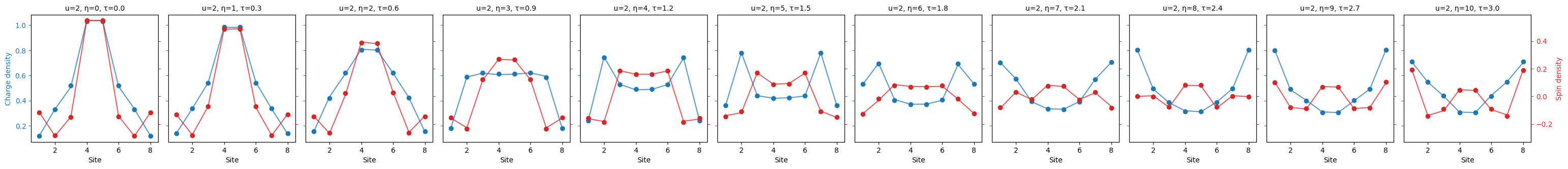
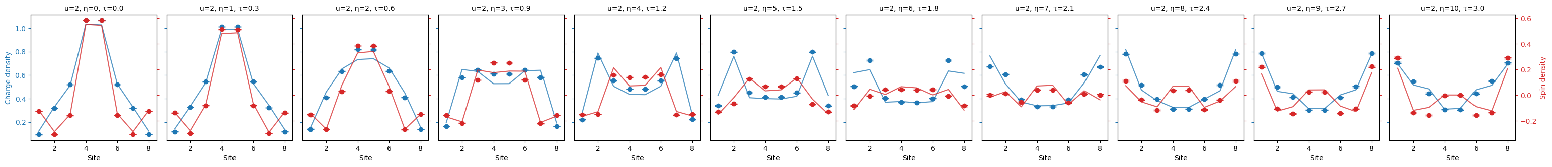
This data frame contains the value, standard error, and standard deviation of the "charge_spin_density" quantity at each site for each time (Trotter step). For convenience, this quantity (and others) can be plotted with the fermi_hubbard.plot_quantity helper function.
"""Plot the charge spin density."""
fermi_hubbard.plot_quantity(bundle, "charge_spin_density");
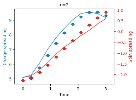
This plotting function automatically adjusts the appearance of plots according to the data being plotted. We illustrate this by plotting the "charge_spin_spreading" below.
"""Plot the charge spin spreading."""
fermi_hubbard.plot_quantity(bundle, "charge_spin_spreading");
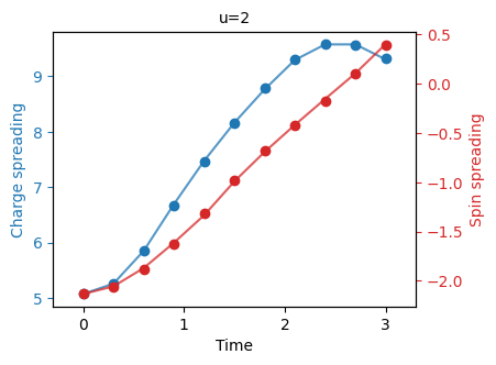
One can compare these plots to Figure 2 of the Fermi-Hubbard experiment paper.
Parasitic controlled-phase
We now run the same experiment but with the google_sqrt_iswap_converter. As mentioned, this decomposes \(\sqrt{\small \mbox{iSWAP} }\) gates imperfectly as cirq.FSim(π/4, π/24) which is close to the average value of the parasitic controlled phase on the Rainbow processor.
"""Run the experiments on a noisy simulator for each qubit layout."""
parasitic_sampler = fermi_hubbard.ConvertingSampler(
    cirq.Simulator(), publication.google_sqrt_iswap_converter().convert
    )

with tqdm(range(len(parameters) * len(trotter_steps))) as progress:
    experiments = [
        fermi_hubbard.run_experiment(
            params,
            trotter_steps,
            parasitic_sampler,
            post_run_func=lambda *_: progress.update()
        )
        for params in parameters
    ]
0%| | 0/176 [00:00<?, ?it/s]
As above, we can post-process the data using an InstanceBundle and plot quantities of interest using the plot_quantity helper function.
"""Post-process the experimental data for all qubit layouts."""
bundle = fermi_hubbard.InstanceBundle(experiments)
bundle.cache_exact_numerics()
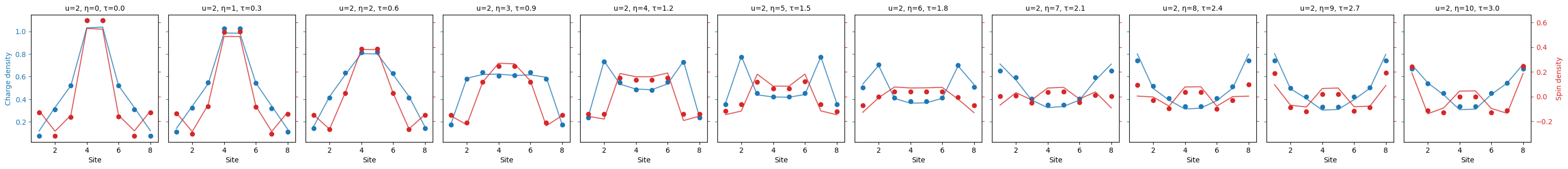
We first plot the "charge_spin_density":
fermi_hubbard.plot_quantity(bundle, "charge_spin_density");
And plot the "charge_spin_spreading" as well.
"""Plot the charge spin spreading."""
fermi_hubbard.plot_quantity(bundle, "charge_spin_spreading", show_std_error=True);
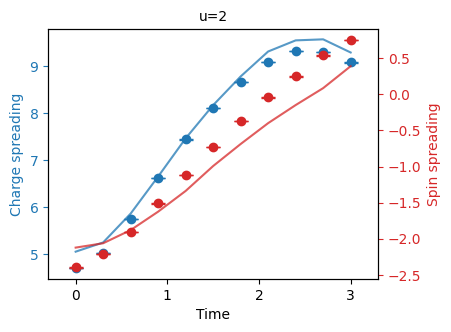
One can compare these to the simulation with exact decompositions above to see the effect of the parasitic controlled phase.
Execution on Google's Quantum Computing Service
In order to run an experiment on Google's QCS, a QuantumEngine sampler is needed. To create an engine sampler, an environment variable GOOGLE_CLOUD_PROJECT must be present and set to a valid Google Cloud Platform project identifier.
"""Get an engine sampler."""
import os
import cirq_google

if "GOOGLE_CLOUD_PROJECT" in os.environ:
    engine_sampler = cirq_google.get_engine_sampler(
        processor_id="rainbow", gate_set_name="sqrt_iswap"
    )
else:
    # Use the simulator as a backup.
    engine_sampler = cirq.Simulator()

# Get a sampler for the Fermi-Hubbard experiment.
google_sampler = fermi_hubbard.ConvertingSampler(
    engine_sampler, publication.google_sqrt_iswap_converter().convert
)
Now that we are running on a quantum computer, we follow good experimental practice and save the results on disk as soon as each experiment finishes using the fermi_hubbard.save_experiment function. Although rare, remote operation may fail for various reasons. More advanced execution workflow might include error handling, experiment pause and continuation, etc., which we omit here for simplicity.
"""Run the experiments on Google's QCS and save the results."""
# Directory to save results in.
results_dir = "trapping"

with tqdm(range(len(layouts) * len(trotter_steps))) as progress:
    for index, params in enumerate(parameters):
        experiment = fermi_hubbard.run_experiment(
            params,
            trotter_steps,
            google_sampler,
            post_run_func=lambda *_: progress.update()
        )

        fermi_hubbard.save_experiment(
            experiment, f"{results_dir}/trapping_{index + 1}.json"
        )
0%| | 0/176 [00:00<?, ?it/s]
We can now load the results using fermi_hubbard.load_experiment.
"""Load experimental results."""
experiments = [
    fermi_hubbard.load_experiment(f"{results_dir}/trapping_{index + 1}.json")
    for index in range(len(parameters))
]
When post-processing experimental data from hardware, we include effects due to the parasitic controlled phase as shown below. The value \(\phi = 0.138\) was the approximate value of the parasitic controlled phase at the time when the experimental results in the paper were collected.
"""Post-process the experimental data for all qubit layouts."""
bundle = fermi_hubbard.InstanceBundle(
    experiments,numerics_transform=publication.parasitic_cphase_compensation(0.138)
)
bundle.cache_exact_numerics()
We can now visualize these results using the same plotting functions from above. Here we show the standard deviation of results in the plots.
"""Plot the charge spin density."""
fermi_hubbard.plot_quantity(bundle, "charge_spin_density", show_std_error=True);
"""Plot the charge spin spreading."""
fermi_hubbard.plot_quantity(bundle, "charge_spin_spreading", show_std_error=True);
If Google's QCS was used, these experimental results can be compared to previous experiments executed on simulators.